LLM Scaling law and Efficiency

• SlideDeck: W11-ScalinglawEfficientLLM
• Version: current
• Lead team: team-4
• Blog team: team-5

In this session, our readings cover:

Required Readings:

Scaling Laws for Neural Language Models

• Jared Kaplan, Sam McCandlish, Tom Henighan, Tom B. Brown, Benjamin Chess, Rewon Child, Scott Gray, Alec Radford, Jeffrey Wu, Dario Amodei

• We study empirical scaling laws for language model performance on the cross-entropy loss. The loss scales as a power-law with model size, dataset size, and the amount of compute used for training, with some trends spanning more than seven orders of magnitude. Other architectural details such as network width or depth have minimal effects within a wide range. Simple equations govern the dependence of overfitting on model/dataset size and the dependence of training speed on model size. These relationships allow us to determine the optimal allocation of a fixed compute budget. Larger models are significantly more sample-efficient, such that optimally compute-efficient training involves training very large models on a relatively modest amount of data and stopping significantly before convergence.

• https://github.com/RUCAIBox/LLMSurvey

Efficient Large Language Models: A Survey

• https://arxiv.org/abs/2312.03863
• https://github.com/AIoT-MLSys-Lab/Efficient-LLMs-Survey
• Large Language Models (LLMs) have demonstrated remarkable capabilities in important tasks such as natural language understanding, language generation, and complex reasoning and have the potential to make a substantial impact on our society. Such capabilities, however, come with the considerable resources they demand, highlighting the strong need to develop effective techniques for addressing their efficiency this http URL this survey, we provide a systematic and comprehensive review of efficient LLMs research. We organize the literature in a taxonomy consisting of three main categories, covering distinct yet interconnected efficient LLMs topics from model-centric, data-centric, and framework-centric perspective, respectively. We have also created a GitHub repository where we compile the papers featured in this survey at this https URL, and will actively maintain this repository and incorporate new research as it emerges. We hope our survey can serve as a valuable resource to help researchers and practitioners gain a systematic understanding of the research developments in efficient LLMs and inspire them to contribute to this important and exciting field.

The Era of 1-bit LLMs: All Large Language Models are in 1.58 Bits

• Recent research, such as BitNet [23], is paving the way for a new era of 1-bit Large Language Models (LLMs). In this work, we introduce a 1-bit LLM variant, namely BitNet b1.58, in which every single parameter (or weight) of the LLM is ternary {-1, 0, 1}. It matches the full-precision (i.e., FP16 or BF16) Transformer LLM with the same model size and training tokens in terms of both perplexity and end-task performance, while being significantly more cost-effective in terms of latency, memory, throughput, and energy consumption. More profoundly, the 1.58-bit LLM defines a new scaling law and recipe for training new generations of LLMs that are both high-performance and cost-effective. Furthermore, it enables a new computation paradigm and opens the door for designing specific hardware optimized for 1-bit LLMs.

More Readings:

An Expert is Worth One Token: Synergizing Multiple Expert LLMs as Generalist via Expert Token Routing

• Ziwei Chai, Guoyin Wang, Jing Su, Tianjie Zhang, Xuanwen Huang, Xuwu Wang, Jingjing Xu, Jianbo Yuan, Hongxia Yang, Fei Wu, Yang Yang
• We present Expert-Token-Routing, a unified generalist framework that facilitates seamless integration of multiple expert LLMs. Our framework represents expert LLMs as special expert tokens within the vocabulary of a meta LLM. The meta LLM can route to an expert LLM like generating new tokens. Expert-Token-Routing not only supports learning the implicit expertise of expert LLMs from existing instruction dataset but also allows for dynamic extension of new expert LLMs in a plug-and-play manner. It also conceals the detailed collaboration process from the user’s perspective, facilitating interaction as though it were a singular LLM. Our framework outperforms various existing multi-LLM collaboration paradigms across benchmarks that incorporate six diverse expert domains, demonstrating effectiveness and robustness in building generalist LLM system via synergizing multiple expert LLMs.

LIMA: Less Is More for Alignment /

• https://arxiv.org/abs/2305.11206
• Large language models are trained in two stages: (1) unsupervised pretraining from raw text, to learn general-purpose representations, and (2) large scale instruction tuning and reinforcement learning, to better align to end tasks and user preferences. We measure the relative importance of these two stages by training LIMA, a 65B parameter LLaMa language model fine-tuned with the standard supervised loss on only 1,000 carefully curated prompts and responses, without any reinforcement learning or human preference modeling. LIMA demonstrates remarkably strong performance, learning to follow specific response formats from only a handful of examples in the training data, including complex queries that range from planning trip itineraries to speculating about alternate history. Moreover, the model tends to generalize well to unseen tasks that did not appear in the training data. In a controlled human study, responses from LIMA are either equivalent or strictly preferred to GPT-4 in 43% of cases; this statistic is as high as 58% when compared to Bard and 65% versus DaVinci003, which was trained with human feedback. Taken together, these results strongly suggest that almost all knowledge in large language models is learned during pretraining, and only limited instruction tuning data is necessary to teach models to produce high quality output.

Blog: Blog Start

Paper 1: Efficient Large Language Models: A Survey

Introduction

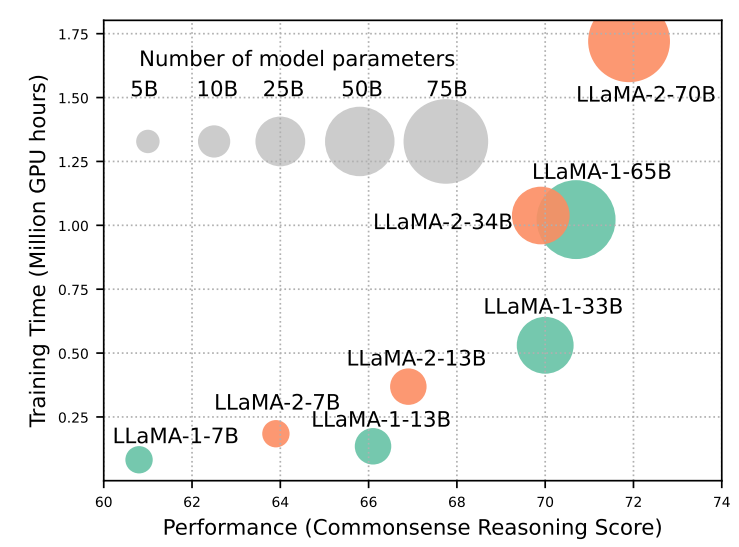
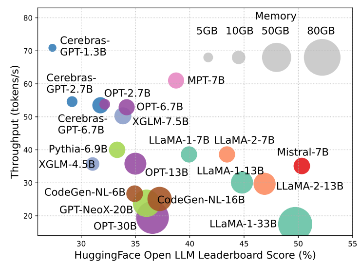
Large Language Models (LLMs) represent a significant advancement in AI, capable of understanding and generating human languages. Prominent examples include OpenAI’s GPT-3 and GPT-4, Google’s Gemini, GLaM, PaLM, and Meta’s LLaMA-1 and LLaMA-2, among others like BLOOM, PanGu-P, and GLM. These models excel in various tasks such as natural language understanding, language generation, complex reasoning, and domain-specific applications like biomedicine, law, and code generation. Their remarkable performance stems from their massive scale, with billions or even trillions of parameters trained on vast and diverse datasets.

However, the impressive capabilities of LLMs come with substantial resource demands, both in terms of training time and inference costs. Larger models achieve better performance but require exponentially more GPU hours for training. Additionally, scaling up model size leads to lower inference throughput, posing challenges for wider adoption and cost-effective application deployment. To address these issues, there’s a pressing need to develop efficiency techniques for LLMs. For instance, Mistral-7B employs grouped-query attention and sliding window attention to enhance inference speed while maintaining comparable performance, demonstrating the feasibility and importance of efficiency optimizations for LLMs.

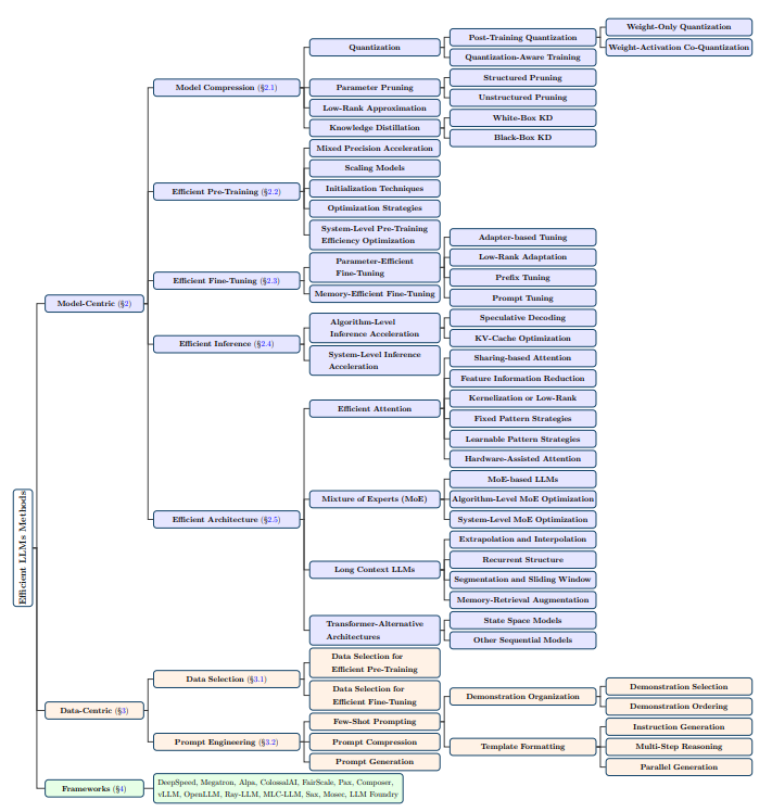
) This survey aims to offer a comprehensive overview of technological advancements in efficient Large Language Models (LLMs) and summarize current research directions. The literature is categorized into three main areas: model-centric, data-centric, and framework-centric perspectives.

• Model-Centric Methods: These methods focus on efficient techniques at both algorithm and system levels, with the model itself as the central focus. Topics covered include model compression, efficient pre-training, fine-tuning, inference, and architecture design.

• Data-Centric Methods: The quality and structure of data are crucial for efficient LLMs. This category explores techniques related to data selection and prompt engineering to enhance efficiency.

• LLM Frameworks: Specialized frameworks have emerged to handle the unique demands of LLMs in training, inference, and serving. While mainstream AI frameworks like TensorFlow and PyTorch provide foundations, specialized frameworks addressing LLM-specific optimizations and features are surveyed, including their unique attributes, underlying libraries, and specializations.

Model Centric Methods:

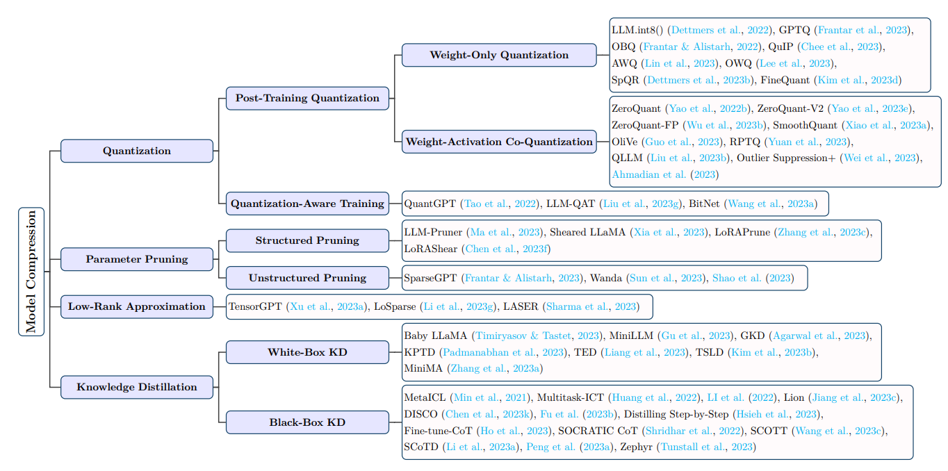
• Model Compression :
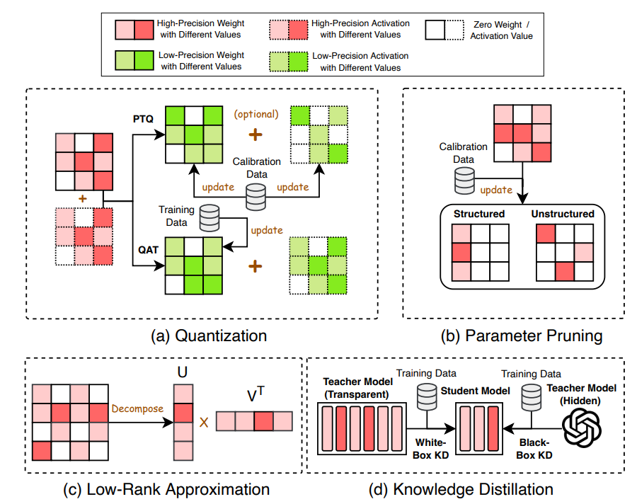
  • Quantization : Quantization is a method to compress Large Language Models (LLMs) by converting their high-precision data types, like 32-bit floating point, into lower precision types, like 8-bit integers. This process involves rounding the values based on the maximum absolute value within the data set.
  • Parameter Pruning : Parameter pruning compresses LLMs by removing redundant model weights. Parameter pruning methods for LLMs can be categorized into structured pruning and unstructured pruning.
  • Low Rank Approximation : Low-rank approximation is a compression technique for Large Language Models (LLMs) where the weight matrix $W_{m \times n}$ is approximated by lower rank matrices $U$ and $V$, such that $W \approx UV^T$, where $U \in R^{m \times r}$, $V \in R^{n \times r}$, and r is usually much smaller than m and n. This method reduces the number of parameters and improves computational efficiency. For instance, TensorGPT by Xu et al. (2023a) employs Tensor-Train Decomposition (TTD) to compress LLMs’ embedding layers, creating an efficient format named Matrix Product State (MPS). LoSparse (Li et al., 2023g) aims to compress neurons’ coherent and expressive components using low-rank approximation while eliminating non-expressive elements through sparse matrix pruning, achieving superior results compared to conventional pruning methods through iterative training and important score calculation.
  • Knowledge Distillation : nowledge Distillation (KD) compresses LLMs by training a smaller student model to emulate the performance of the LLM as the teacher model such that the student model is computationally less expansive yet maintains a high level of performance similar to the teacher model. KD for LLMs can be categorized into white-box KD methods and black-box KD methods
    • White-Box : White-box Knowledge Distillation (KD) involves using the parameters or logits of the teacher Large Language Model (LLM) in the distillation process. For instance, Baby LLaMA trains an ensemble of GPT-2 and smaller LLaMA-1 models using a dataset of 10M words, then distills them into a compact LLaMA model with 58 million parameters, outperforming both its original teacher models and a comparable model trained without distillation. MiniLLM minimizes reverse Kullback-Leibler divergence using policy gradient techniques, surpassing standard KD benchmarks on a 13-billion-parameter LLaMA-1 model. Generalized Knowledge Distillation (GKD) addresses distribution mismatch by drawing output sequences from the student model during training and optimizing different divergence measures like reverse KL to produce samples probable within the teacher model’s distribution. KPTD successfully transfers knowledge from entity definitions into the parameters of a pre-trained language model, while TED introduces layer-specific task distillation by aligning internal states of student and teacher models in each layer using specially designed filters.
    • Black-Box : In black-box Knowledge Distillation (KD), only the outputs generated from the teacher Large Language Model (LLM) are utilized in the distillation process. Multitask-ICT introduces in-context learning distillation to transfer few-shot learning capabilities from the LLM teacher to the student model. LI et al. employ a hybrid prompting technique to distill explanations into smaller models, achieving consistent improvements over single-task fine-tuning benchmarks. Lion introduces an adversarial distillation architecture to incrementally improve the student model’s skill level. DISCO prompts a general LLM to produce phrasal perturbations, filtered by a specialized teacher model to distill high-quality counterfactual data into smaller student models. Fu et al. aim to enhance smaller models’ complex reasoning abilities through chain-of-thought prompting, utilizing instruct-tuning from a LLM teacher to generalize well to new scenarios.

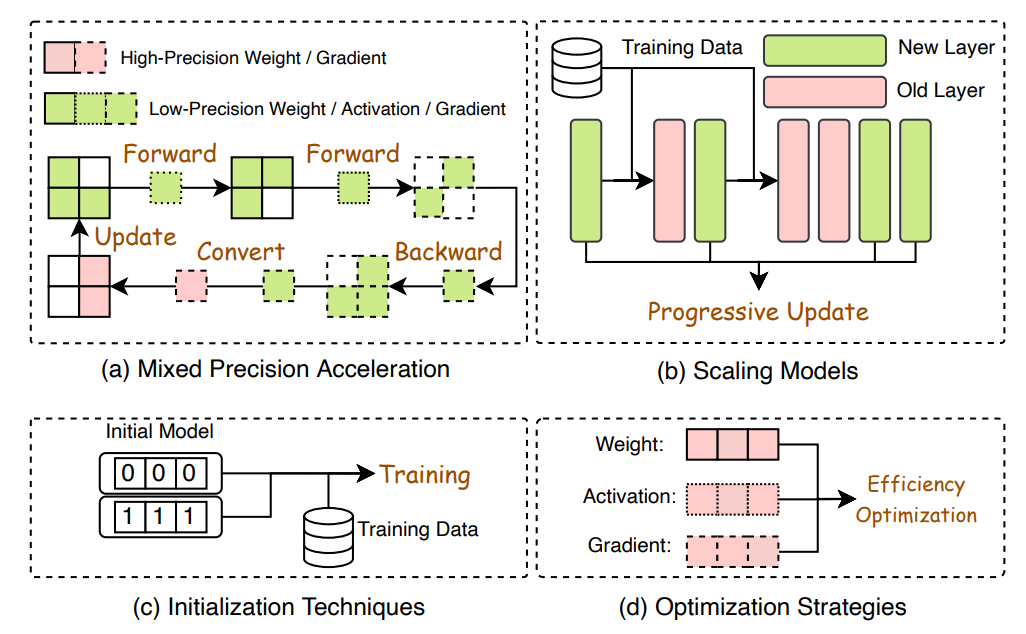
• Efficient Pretraining : fficient pre-training of Large Language Models (LLMs) aims to reduce costs. Techniques include mixed precision acceleration, scaling models, initialization techniques, and optimization strategies. Mixed precision acceleration utilizes low-precision models for forward and backward propagation, then converts gradients to high precision for weight updates. Scaling models transfer knowledge from smaller to larger models, employing techniques like Progressive Stacking and CompoundGrow. Initialization techniques ensure stable convergence of models, such as Fixup and ReZero. Optimization strategies, like Lion and Sophia, propose memory-efficient optimizers. System-level efficiency optimization focuses on distributed training methods such as data parallelism, pipeline parallelism, and tensor parallelism. Techniques like ZeRO and FSDP optimize memory usage and communication overhead during training across multiple compute nodes.

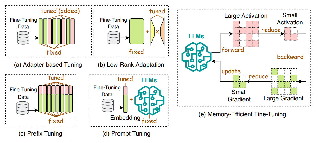
• Efficient Fine Tuning : Efficient fine-tuning improves the adaptation of LLMs to downstream tasks, with methods categorized into parameter-efficient fine-tuning (PEFT) and memory-efficient fine-tuning (MEFT). PEFT involves freezing the LLM backbone and updating only a subset of parameters, including adapter-based tuning, low-rank adaptation, prefix tuning, and prompt tuning. Adapter-based tuning integrates trainable adapter modules into LLMs, while low-rank adaptation updates small matrices to enhance efficiency. Prefix tuning adds trainable vectors to LLM layers, and prompt tuning inserts trainable prompt tokens at the input layer. These techniques optimize fine-tuning processes for improved task performance.

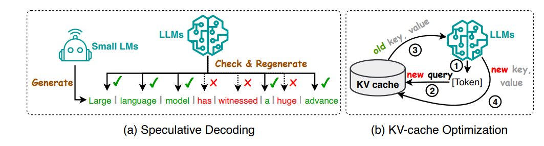
• Efficient Inference : Efficient inference for LLMs focuses on optimizing speed and resource utilization, categorized into algorithm-level and system-level techniques. Algorithm-level optimizations include speculative decoding, which speeds up sampling by using smaller models to create speculative prefixes, and KV-cache optimization, which minimizes repeated computation of Key-Value pairs. System-level optimizations involve techniques like FlexGen, which coordinates hardware resources for high-throughput inference on GPUs with limited memory, and S3, which optimizes resource utilization by anticipating output sequence length. These methods collectively enhance LLM inference efficiency for diverse applications.

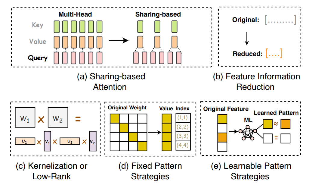
• Efficient Architecture : Efficient architecture design for LLMs involves optimizing model architecture and computational processes to improve performance while minimizing resource consumption. Techniques for efficient attention include sharing-based attention, feature information reduction, kernelization or low-rank methods, fixed pattern strategies, learnable pattern strategies, and hardware-assisted attention. Sharing-based attention optimizes computation by sharing keys and values across multiple query heads, while feature information reduction reduces computational demands by compressing sequence representations. Kernelization and low-rank techniques compact attention matrices for faster computation, while fixed pattern strategies confine attention to predetermined patterns, improving efficiency. Learnable pattern strategies group tokens into clusters to enhance efficiency, and hardware-assisted attention focuses on optimizing attention computation from a hardware perspective. These approaches collectively contribute to more efficient and scalable LLM architectures.

Data Centric Methods :

• Prompt Engineering : Prompt engineering, as proposed by Liu et al. (2023c), focuses on optimizing input prompts to guide LLMs in generating desired outputs, thereby enhancing inference efficiency. This approach tailors prompts or queries to better align with the capabilities and nuances of specific language models. In some cases, like semantic classification, prompt engineering can even replace fine-tuning while achieving high accuracy (Liu et al., 2022b). Techniques in prompt engineering include few-shot prompting, prompt compression, and prompt generation, which collectively contribute to improving the effectiveness and efficiency of LLMs.

  • Few-Shot Prompting : Few-shot prompting involves providing an LLM with a limited set of examples (demonstrations) to guide its understanding of a task it needs to perform (Wei et al., 2022a). These demonstrations, selected based on their similarity to the test example, enable the LLM to utilize the knowledge gained from them to make accurate predictions. Few-shot prompting enhances inference efficiency by allowing LLMs to perform various tasks without additional training or fine-tuning. Techniques in few-shot prompting include demonstration selection, demonstration ordering, instruction generation, and multi-step reasoning.

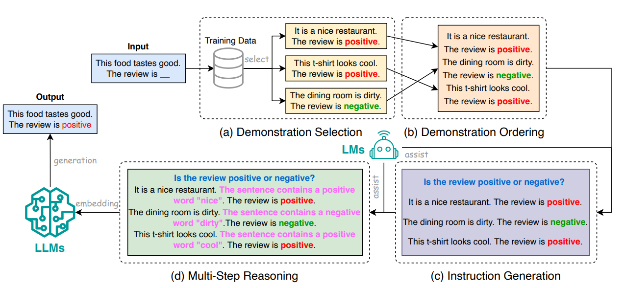
 + Demonstration selection : Involves choosing representative examples for prompting, either through unsupervised methods like nearest neighbor selection or supervised methods 
   involving training domain-specific retrievers. Demonstration ordering arranges selected demonstrations to form an appropriate prompt, impacting the model's performance. 
   Template formatting focuses on designing concise templates for prompts, including instruction generation to provide task context and multi-step reasoning to guide LLMs 
   through intermediate steps.

 + Multi-step reasoning : Also known as Chain-of-Thought (CoT) prompting, guides LLMs through a sequence of intermediate steps before producing the final answer, enhancing 
   generation quality. Techniques like Auto-CoT, Self-Ask, ReAct, Least-to-Most Prompting, Tree-of-Thought, and Contrastive CoT address challenges in multi-step reasoning,   ensuring accurate reasoning processes. Parallel generation accelerates inference by guiding LLMs to first generate an answer template and then complete it simultaneously, enhancing hardware utilization and speed. Overall, few-shot prompting techniques improve inference efficiency by effectively guiding LLMs through tasks with minimal examples and optimized prompts

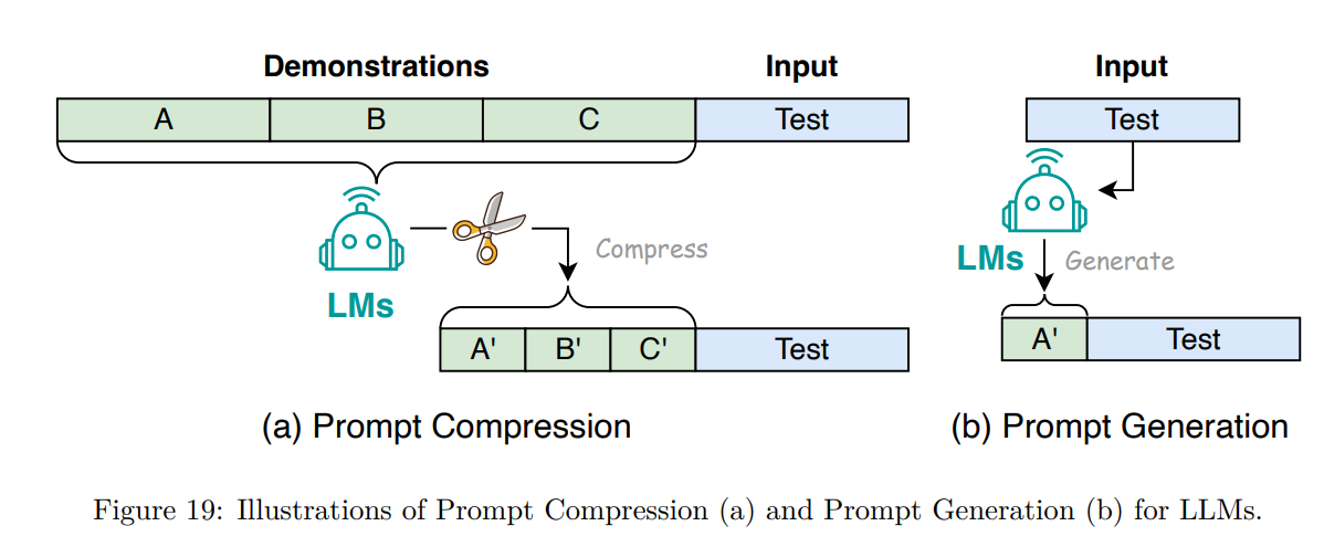
• Prompt Compression and Generation : Prompt compression techniques accelerate the processing of LLM inputs by condensing lengthy prompts or learning compact representations. Mu et al. propose distilling prompts into concise gist tokens, reducing prompts by up to 26 times and FLOPs by up to 40%. AutoCompressors by Chevalier et al. condense long contexts into summary vectors, extending the model’s context window with less computational cost. PCRL by Jung & Kim employs reinforcement learning to edit prompts, achieving a 24.6% average reduction in token count. ICAE by Ge et al. compresses context into memory slots, achieving 4x compression. Nugget 2D represents historical context as compact nuggets, and LongLLMLingua introduces question-aware compression techniques. Prompt generation enhances efficiency by automatically creating effective prompts for LLMs. AutoPrompt proposes a gradient-guided search method for prompt generation across tasks, emphasizing the role of human-written text in optimizing LLM performance. TempLM combines generative and template-based approaches for data-to-text tasks. PromptGen dynamically generates prompts for knowledge probing tasks based on pre-trained LLMs, outperforming AutoPrompt on benchmarks. )

LLM Frameworks :

Here are short bullet point type descriptions of some of the LLM frameworks

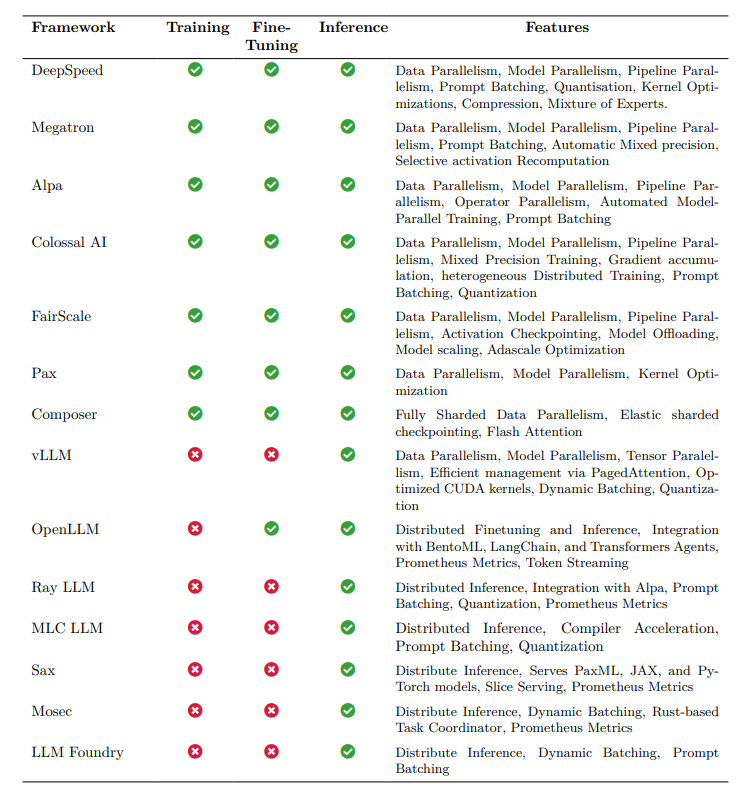
• DeepSpeed: Developed by Microsoft for training and deploying LLMs. Includes DeepSpeed-Inference foundational library. Features ZeRO-Inference to address GPU memory constraints, deep fusion mechanism, and DeepSpeed Model Implementations for Inference (DeepSpeed MII). DeepSpeed-Chat adds chat support, integrating techniques from Reinforcement Learning from Human Feedback (RLHF).
• Megatron: Nvidia’s framework for training and deploying LLMs. Used for Nvidia’s Megatron models. Utilizes strategic decomposition of tensor operations across multiple GPUs, FasterTransformer for optimizing inference, and TensorRT-LLM for reducing latency.
• Alpa: Library for training and serving large-scale neural networks. Addresses inter- and intra-operator parallelism, with example implementations for various models. Core methodology includes automatic parallelization and integrated design combining data and model parallelism.
• ColossalAI: A unified solution for large-scale distributed training. Provides implementations for various LLMs and emphasizes holistic integration of deep learning pipelines. Modular architecture and integration of advanced optimization techniques.
• FairScale: Developed by Meta for high-performance and large-scale training with PyTorch. Focuses on usability, modularity, and performance. Supports Fully Sharded Data Parallel (FSDP) and features activation checkpointing, model offloading, and scaling.
• Pax: Google’s JAX-based efficient distributed training framework. Used for training models across modalities. Key components include SeqIO, Optax, Fiddle, Orbax, PyGLove, and Flax.
• Composer: Developed by Mosaic ML for faster and more efficient neural network training. Supports FSDP, elastic shared checkpointing, and dataset streaming. Designed with both Functional and Trainer APIs for versatility and ease of use.
• vLLM: Represents a methodological shift in LLM serving, with a focus on memory management efficiency. Features PagedAttention, adaptive loading technique, and parameter compression strategy. Supports state-of-the-art quantization techniques and optimized CUDA kernels.
• OpenLLM: A comprehensive approach to deploying LLMs in production environments within the BentoML ecosystem. Emphasizes modularity, scalability, and advanced caching mechanisms for optimized operational costs and response times.
• Ray-LLM: Integration of LLMs with the Ray ecosystem for optimized deployment and operation. Leverages Ray’s distributed computing capabilities for efficient task scheduling and execution. Designed for enhanced model performance, reduced latency, and optimized resource utilization.
• MLC-LLM: Empowers individuals to develop, optimize, and deploy AI models on diverse devices. Focuses on device-native AI, optimizing models for specific device capabilities and constraints. Demonstrates state-of-the-art performance in terms of throughput across various devices.
• Sax: Designed by Google for deploying Pax, JAX, and PyTorch models for inference tasks. Sax cell comprises an administrative server and multiple model servers for efficient model serving. Complementary to the Pax framework, geared toward model serving.
• Mosec: Streamlines the serving of large deep learning models, particularly in cloud environments. Features high performance with Rust-built web layer and task coordination, dynamic batching, and cloud-friendly capabilities.
• LLM Foundry: Library for finetuning, evaluating, and deploying LLMs for inference with Composer and the MosaicML platform. Supports distributed inference, dynamic batching, and prompt batching for efficient deployment. Designed for easy use, efficiency, and flexibility, enabling rapid experimentation with the latest LLM techniques.

Paper 2: Scaling Laws for Neural Language Models

Introduction

The study emphasizes language as a natural domain for artificial intelligence research due to its suitability for expressing and evaluating reasoning tasks. Recent advancements in deep learning, particularly in language modeling, have led to models approaching human-level performance on various tasks, including generating coherent text samples. The study aims to empirically investigate how language modeling performance is affected by factors such as model architecture, model size, computing power, and dataset size. The analysis focuses on the Transformer architecture and observes precise power-law scalings for performance concerning training time, context length, dataset size, model size, and compute budget.

Summary of Findings :

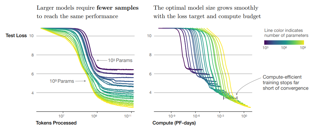
The study finds that model performance in language modeling strongly depends on scale factors, particularly the number of model parameters, dataset size, and compute used for training. These factors exhibit smooth power-law relationships with performance over a wide range of scales. Performance improves predictably when both model size and dataset size are increased together, but diminishes returns occur when only one factor is increased while the other is held fixed. Training curves follow predictable power laws, allowing for rough predictions of performance with longer training. Transfer to different distributions incurs a constant penalty but otherwise improves roughly in line with training set performance. Large models are more sample-efficient and converge optimally by training very large models and stopping short of convergence. The optimal batch size for training is roughly determined by measuring the gradient noise scale. Overall, scaling up model size, data, and compute leads to smooth and predictable improvements in language modeling performance and sample efficiency.

Summary of Scaling Laws :

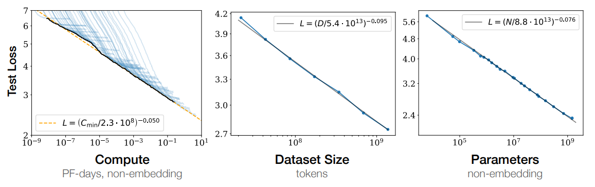
The test loss of a Transformer trained to autoregressively model language can be predicted using a power-law when performance is limited by only either the number of non-embedding parameters $N$, the dataset size $D$, or the optimally allocated compute budget $ C_{\text{min}}$

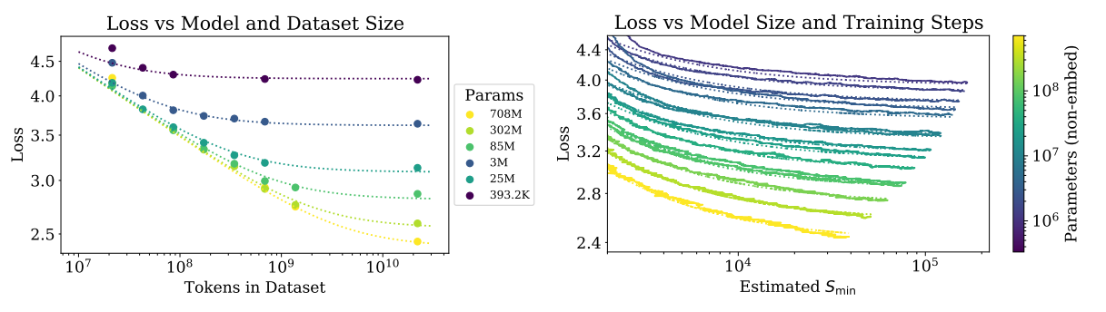
Left: The early-stopped test loss $L(N, D)$ varies predictably with the dataset size $D$ and model size $N$ according to Equation (1.5). Right: After an initial transient period, learning curves for all model sizes $N$ can be fit with Equation (1.6), which is parameterized in terms of $S_{min}$, the number of steps when training at large batch size

1. For models with a limited number of parameters, trained to convergence on sufficiently large datasets: \(L(N) = \left( \frac{N_c}{N} \right)^{\alpha_N}; \quad \alpha_N \approx 0.076, \quad N_c \approx 8.8 \times 10^{13}\)

2. For large models trained with a limited dataset with early stopping: \(L(D) = \left( \frac{D_c}{D} \right)^{\alpha_D}; \quad \alpha_D \approx 0.095, \quad D_c \approx 5.4 \times 10^{13}\)

3. When training with a limited amount of compute, a sufficiently large dataset, an optimally-sized model, and a sufficiently small batch size (making optimal3 use of compute): \(L(C_{\text{min}}) =\)

4. The critical batch size, which determines the speed/efficiency tradeoff for data parallelism: \(B_{\text{crit}}(L) = B^* \cdot L^{\frac{1}{\alpha_B}}; \quad B^* \approx 2 \times 10^8, \quad \alpha_B \approx 0.21\)

5. The equation combining (1.1) and (1.2) that governs the simultaneous dependence on $N$ and $D$ and governs the degree of overfitting: \(L(N, D) = \left( \frac{N_c}{N} \right)^{\alpha_N \alpha_D} + \left( \frac{D_c}{D} \right)^{\alpha_D}\)

6. When training a given model for a finite number of parameter update steps $S$ in the infinite data limit: \(L(N, S) = \left( \frac{N_c}{N} \right)^{\alpha_N} + \left( \frac{S_c}{S_{\text{min}}(S)} \right)^{\alpha_S}; \quad S_c \approx 2.1 \times 10^3, \quad \alpha_S \approx 0.76\)

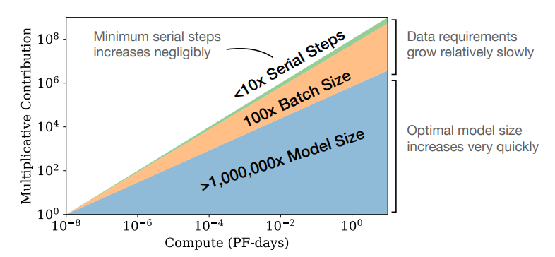
7. When training within a fixed compute budget $C$, but with no other constraints: \(N \propto C_{\text{min}}^{\frac{1}{\alpha}}\) \(B \propto C_{\text{min}}^{\frac{1}{\alpha_B}}\) \(S \propto C_{\text{min}}^{\frac{1}{\alpha_S}}\) \(D = B \cdot S\)

8. The calculation for $\alpha_{\text{min}}$: \(\alpha_{\text{min}} = \frac{1}{\left( \frac{1}{\alpha_S} + \frac{1}{\alpha_B} + \frac{1}{\alpha_N} \right)}\)

Notation :

We use the following notation:

• $L$ – the cross entropy loss in nats. Typically it will be averaged over the tokens in a context, but in some cases we report the loss for specific tokens within the context.
• $N$ – the number of model parameters, excluding all vocabulary and positional embeddings
• $C \approx 6NBS$ – an estimate of the total non-embedding training compute, where $B$ is the batch size, and $S$ is the number of training steps (i.e., parameter updates). We quote numerical values in PF-days, where one PF-day = $10^{15} \times 24 \times 3600 = 8.64 \times 10^{19}$ floating-point operations.
• $D$ – the dataset size in tokens
• $B_{\text{crit}}$ – the critical batch size [MKAT18], defined and discussed in Section 5.1. Training at the critical batch size provides a roughly optimal compromise between time and compute efficiency.
• $C_{\text{min}}$ – an estimate of the minimum amount of non-embedding compute to reach a given value of the loss. This is the training compute that would be used if the model were trained at a batch size much less than the critical batch size.
• $S_{\text{min}}$ – an estimate of the minimal number of training steps needed to reach a given value of the loss. This is also the number of training steps that would be used if the model were trained at a batch size much greater than the critical batch size.
• $\alpha_X$ – power-law exponents for the scaling of the loss as $L(X) \propto \frac{1}{X^{\alpha_X}}$ where $X$ can be any of $N$, $D$, $C$, $S$, $B$, $C_{\text{min}}$.

Model Performance :

To characterize language model scaling we train a wide variety of models, varying a number of factorsincluding: • Model size (ranging in size from 768 to 1.5 billion non-embedding parameters) • Dataset size (ranging from 22 million to 23 billion tokens) • Shape (including depth, width, attention heads, and feed-forward dimension) • Context length (1024 for most runs, though we also experiment with shorter contexts) • Batch size (219 for most runs, but we also vary it to measure the critical batch size)

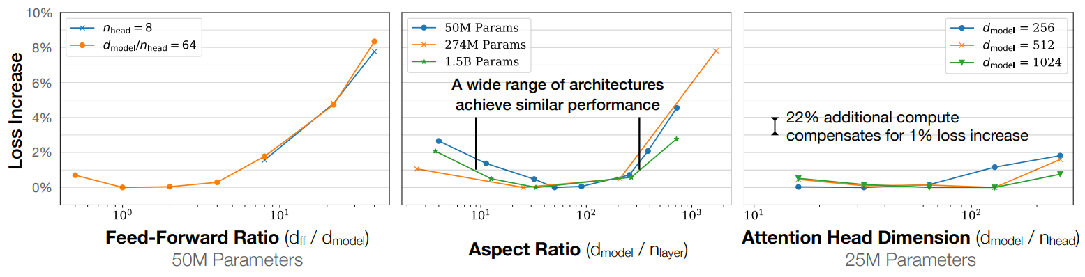
Performance depends very mildly on model shape when the total number of non-embedding parameters N is held fixed. The loss varies only a few percent over a wide range of shapes. Small differences in parameter counts are compensated for by using the fit to L(N) as a baseline. Aspect ratio in particular can vary by a factor of 40 while only slightly impacting performance; an $(n_{layer}, d_{model}) = (6, 4288)$ reaches a loss within 3% of the (48, 1600) model used in [RWC+19].

Transformer performance exhibits weak dependence on the architectural parameters such as the number of layers $n_{layer}$, the number of attention heads $n_{heads}$, and the feed-forward dimension $d_{ff}$, provided that the total non-embedding parameter count $N$ remains fixed. To verify this, experiments were conducted by keeping one hyperparameter fixed while varying another. For instance, when investigating $n_{heads}$, models with fixed size were trained, and only the number of attention heads was altered. Similarly, experiments involving $n_{layer}$ and $d_{ff}$ were conducted by adjusting $d_{model}$ accordingly to maintain a constant $N \approx 12 \times n_{layer} \times d_{model}^{2}$. The observed weak sensitivity to these shape parameters suggests that deeper Transformers may function akin to ensembles of shallower models, analogous to observations made with ResNets.

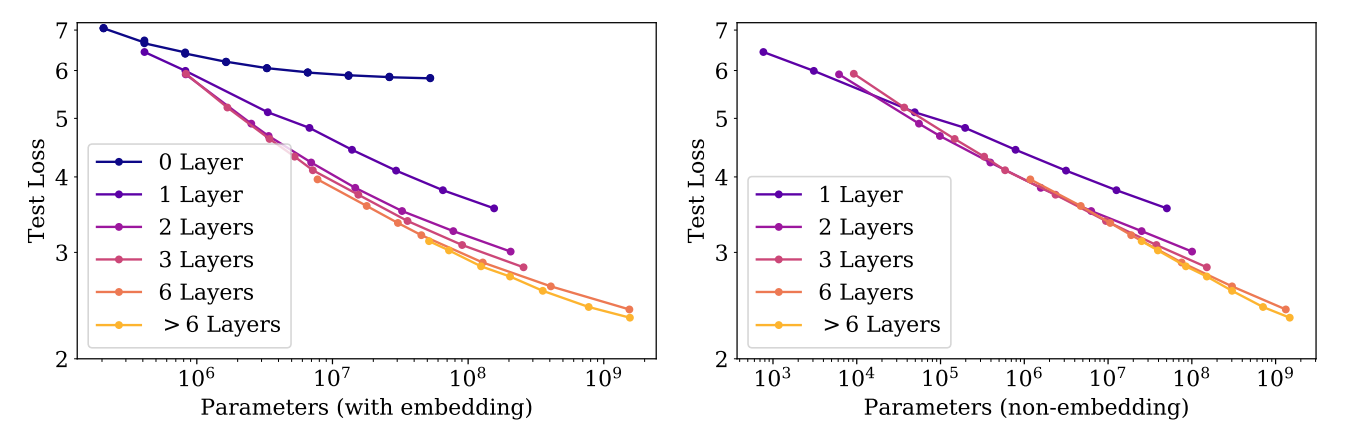
Left: When we include embedding parameters, performance appears to depend strongly on the number of layers in addition to the number of parameters. Right: When we exclude embedding parameters, the performance of models with different depths converge to a single trend. Only models with fewer than 2 layers or with extreme depth-to-width ratios deviate significantly from the trend.

The trend observed with the non-embedding parameter count $N$ follows a steady pattern, which can be approximated by the first term of Equation (1.5), yielding:

$L(N) \approx \left( \frac{N_c}{N} \right)^{\alpha_N}$

To understand these patterns, it’s essential to analyze performance concerning $N$. When considering the total parameter count, including embedding parameters, the trend becomes somewhat unclear. This implies that the embedding matrix’s size can potentially be reduced without affecting performance, as demonstrated in recent studies. Despite being trained on the WebText2 dataset, these models exhibit test loss trends on various other datasets that also follow a power-law in $N$ with nearly identical powers.

Proposed Equation:

We have chosen the parameterization (1.5) (repeated here for convenience):

1. Changes in vocabulary size or tokenization are expected to rescale the loss by an overall factor. The parameterization of $L(N, D)$ (and all models of the loss) must naturally allow for such a rescaling.

2. Fixing $D$ and sending $N \rightarrow \infty$, the overall loss should approach $L(D)$. Conversely, fixing $N$ and sending $D \rightarrow \infty$, the loss must approach $L(N)$.

3. $L(N, D)$ should be analytic at $D = \infty$, so that it has a series expansion in $\frac{1}{D}$ with integer powers. Theoretical support for this principle is significantly weaker than for the first two.

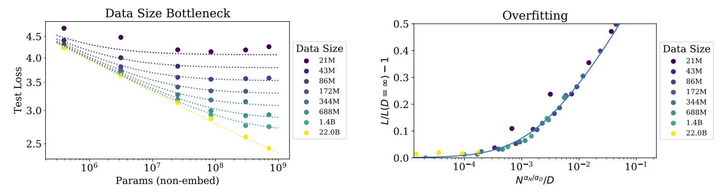
The early-stopped test loss $L(N, D)$ depends predictably on the dataset size $D$ and model size $N$ according to Equation (1.5).

Left: For large $D$, performance is a straight power law in $N$. For a smaller fixed $D$, performance stops improving as $N$ increases and the model begins to overfit. (The reverse is also true, see Figure 4.). Right: The extent of overfitting depends predominantly on the ratio $\frac{N \alpha}{N \alpha D} / D$, as predicted in equation (4.3). The line is our fit to that equation.

Our choice of $L(N, D)$ satisfies the first requirement because we can rescale $Nc$, $Dc$ with changes in the vocabulary. This also implies that the values of $Nc$, $Dc$ have no fundamental meaning.

Since we stop training early when the test loss ceases to improve and optimize all models in the same way, we expect that larger models should always perform better than smaller models. But with fixed finite $D$, we also do not expect any model to be capable of approaching the best possible loss (i.e., the entropy of text). Similarly, a model with fixed size will be capacity-limited. These considerations motivate our second principle. Note that knowledge of $L(N)$ at infinite $D$ and $L(D)$ at infinite $N$ fully determines all the parameters in $L(N, D)$.

The third principle is more speculative. There is a simple and general reason one might expect overfitting to scale $\propto \frac{1}{D}$ at very large \(D\). Overfitting should be related to the variance or the signal-to-noise ratio of the dataset, and this scales as $\frac{1}{D}$. This expectation should hold for any smooth loss function since we expect to be able to expand the loss about the $D \rightarrow \infty$ limit. However, this argument assumes that $\frac{1}{D}$ corrections dominate over other sources of variance, such as the finite batch size and other limits on the efficacy of optimization. Without empirical confirmation, we would not be very confident of its applicability. Our third principle explains the asymmetry between the roles of $N$ and $D$ in Equation (1.5). Very similar symmetric expressions are possible, but they would not have a $\frac{1}{D}$ expansion with integer powers and would require the introduction of an additional parameter.

In any case, we will see that our equation for $L(N, D)$ fits the data well, which is the most important justification for our $L(N, D)$ ansatz.

Optimal Allocation of the Compute Budget :

We displayed the empirical trend of performance as a function of the computation used during training in the top-right of Figure 1. However, this result involved training at a fixed batch size $B$, whereas we know that in fact we could train more efficiently by training at the batch size $B_{\text{crit}}$ discussed in Section 5.1. Large and small values of the loss could have been achieved with fewer samples or fewer steps, respectively, and correcting for this inefficiency by standardizing to the critical batch size results in cleaner and more predictable trends.In this section, we will adjust for this oversight. More importantly, we will use the results of Section 5 to determine the optimal allocation of compute between model size $N$ and the quantity of data processed during training, namely $2B_{\text{crit}}S_{\text{min}}$. We will determine this allocation both empirically and theoretically, by using the equation for $L(N, S_{\text{min}})$, and we will demonstrate that these methods agree.

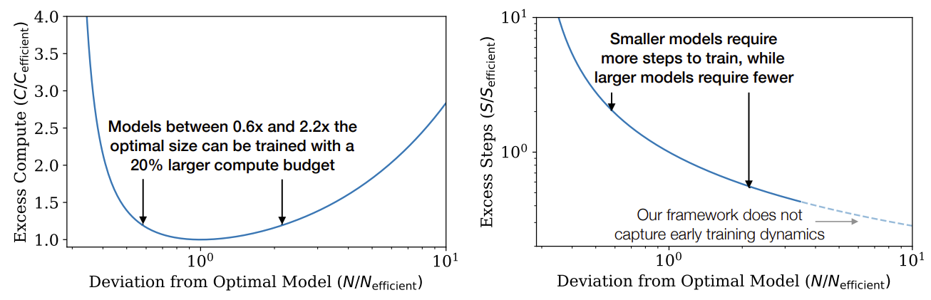
Left: Given a fixed compute budget, a particular model size is optimal, though somewhat larger or smaller models can be trained with minimal additional compute. Right: Models larger than the compute efficient size require fewer steps to train, allowing for potentially faster training if sufficient additional parallelism is possible. Note that this equation should not be trusted for very large models, as it is only valid in the power-law region of the learning curve, after initial transient effects

Conclusion:

We have observed consistent scalings of language model log-likelihood loss with non-embedding parameter count $N$, dataset size $D$, and optimized training computation $C_{\text{min}}$, as encapsulated in Equations (1.5) and (1.6). Conversely, we find very weak dependence on many architectural and optimization hyperparameters. Since scalings with $N$, $D$, $C_{\text{min}}$ are power-laws, there are diminishing returns with increasing scale.

Defining words using the wc utility, the WebText2 dataset has 1.4 tokens per word and 4.3 characters per token. After this work was completed, [RRBS19a] also appeared, which makes similar predictions for the dependence of loss on both model and dataset size.

We were able to precisely model the dependence of the loss on $N$ and $D$, and alternatively on $N$ and $S$, when these parameters are varied simultaneously. We used these relations to derive the compute scaling, magnitude of overfitting, early stopping step, and data requirements when training large language models. So our scaling relations go beyond mere observation to provide a predictive framework. One might interpret these relations as analogues of the ideal gas law, which relates the macroscopic properties of a gas in a universal way, independent of most of the details of its microscopic constituents.

It is natural to conjecture that the scaling relations will apply to other generative modeling tasks with a maximum likelihood loss, and perhaps in other settings as well. To this purpose, it will be interesting to test these relations on other domains, such as images, audio, and video models, and perhaps also for random network distillation. At this point we do not know which of our results depend on the structure of natural language data, and which are universal. It would also be exciting to find a theoretical framework from which the scaling relations can be derived: a ‘statistical mechanics’ underlying the ‘thermodynamics’ we have observed. Such a theory might make it possible to derive other more precise predictions and provide a systematic understanding of the limitations of the scaling laws.

In the domain of natural language, it will be important to investigate whether continued improvement on the loss translates into improvement on relevant language tasks. Smooth quantitative change can mask major qualitative improvements: “more is different”. For example, the smooth aggregate growth of the economy provides no indication of the specific technological developments that underwrite it. Similarly, the smooth improvements in language model loss may hide seemingly qualitative changes in capability.

Our results strongly suggest that larger models will continue to perform better and will also be much more sample efficient than has been previously appreciated. Big models may be more important than big data. In this context, further investigation into model parallelism is warranted. Deep models can be trained using pipelining [HCC+18], which splits parameters depth-wise between devices, but eventually requires increased batch sizes as more devices are used. Wide networks, on the other hand, are more amenable to parallelization [SCP+18], since large layers can be split between multiple workers with less serial dependency. Sparsity [CGRS19, GRK17] or branching (e.g., [KSH12]) may allow for even faster training of large networks through increased model parallelism. And using methods like [WRH17, WYL19], which grow networks as they train, it might be possible to remain on the compute-efficient frontier for an entire training run.

Paper 3: LIMA: Less Is More for Alignment

Introduction

This paper discusses the use of language models trained at a large scale for various language understanding and generation tasks. Alignment methods have been proposed to fine-tune these models for specific tasks, typically requiring significant compute and specialized datasets. However, the authors demonstrate that strong performance can be achieved with just 1,000 carefully curated training examples. The hypothesis is that alignment involves the model learning how to interact with users in terms of style or format, leveraging knowledge acquired during pretraining. To test this, the authors curate examples approximating real user prompts and responses, including questions and answers from community forums and manually written prompts and responses. They then fine-tune a large pretrained model, LIMA, on this dataset.

Comparative evaluations against other models show that LIMA outperforms some state-of-the-art models in human preference studies, achieving equal or preferable responses in a significant percentage of cases. A detailed analysis of LIMA’s responses reveals high adherence to prompt requirements and a considerable proportion of excellent responses. Further experiments highlight the importance of prompt diversity and data quality over sheer quantity in improving model performance. Additionally, despite lacking dialogue examples, LIMA shows competence in conducting coherent multi-turn dialogues, which can be significantly enhanced with a small number of hand-crafted dialogue chains added to the training data.

Overall, these findings underscore the effectiveness of pretraining compared to other approaches such as large-scale instruction tuning and reinforcement learning, showcasing the potential of pretrained models even with limited fine-tuning data.

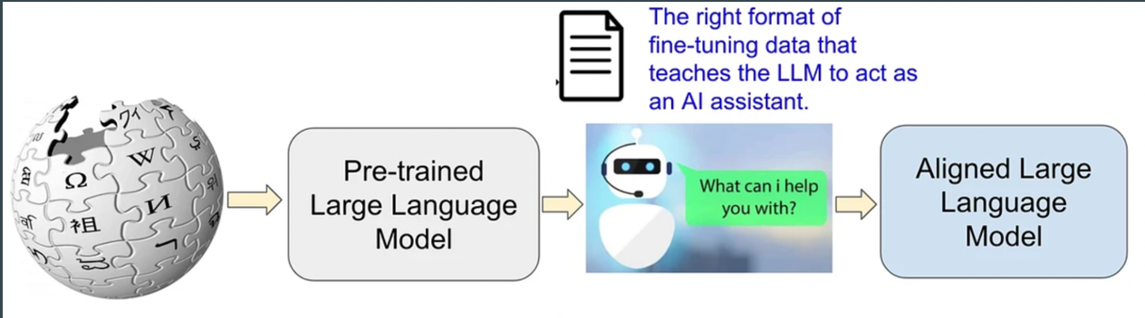
Alignment : Superficial Alignment Hypothesis

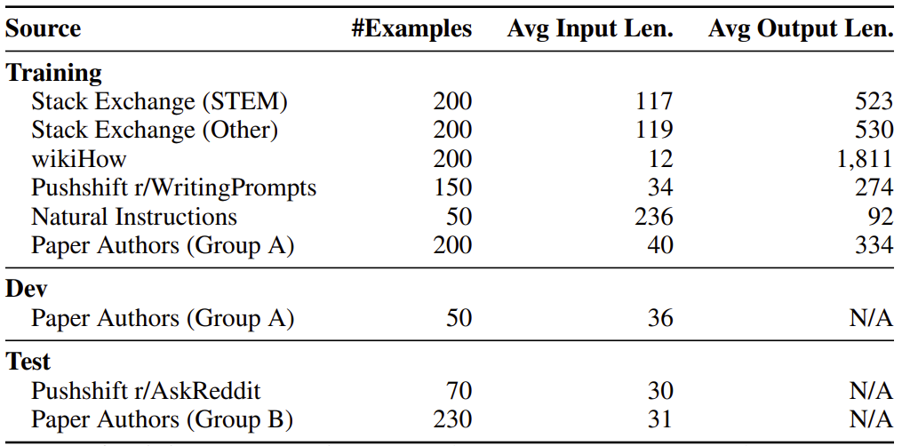
The Superficial Alignment Hypothesis posits that a model’s knowledge and capabilities are predominantly acquired during pretraining, while alignment primarily teaches the model which distribution of formats to utilize when interacting with users. If this hypothesis holds true, and alignment is mainly about learning style, then a corollary suggests that a pretrained language model could be adequately fine-tuned with a relatively small set of examples. To explore this, the authors gather a dataset comprising 1,000 prompts and responses. The responses exhibit stylistic alignment with each other, while the prompts are diverse. These examples are sourced from various platforms, primarily community Q&A forums and manually created instances. Additionally, a test set of 300 prompts and a development set of 50 are collected for evaluation purposes. Table 1 provides an overview of the different data sources along with some statistics.

Alightment Data Types

The Superficial Alignment Hypothesis suggests that a language model primarily learns during pretraining and alignment mainly teaches it which format to use when interacting with users. Hence, fine-tuning with a small set of examples may be sufficient. To test this, the authors collect 1,000 prompts and responses where responses are stylistically aligned but prompts are diverse. These are sourced from community Q&A forums and manually authored examples. A test set of 300 prompts and a development set of 50 are collected. Data from Stack Exchange, wikiHow, and Reddit are mined, with Stack Exchange and wikiHow providing well-aligned content suitable for automated extraction, while Reddit requires manual curation due to its more casual nature. Manually authored examples are diversified further, including natural language generation tasks and prompts with varying tones. This manual curation aims to enhance diversity and quality in contrast to automatic methods that prioritize quantity.

Training LIMA

LIMA (Less Is More for Alignment) is trained using the LLaMa 65B model and fine-tuned on a 1,000-example alignment training set. A special end-of-turn token (EOT) is introduced to differentiate between speakers. Standard fine-tuning hyperparameters are followed, including 15 epochs of training using AdamW optimizer, with batch size set to 32 examples. Residual dropout is applied, starting at 0.0 at the bottom layer and linearly increasing to 0.3 at the last layer. Manual selection of checkpoints is performed based on development set evaluation. LIMA is evaluated against state-of-the-art models and demonstrates superior performance compared to RLHF-based DaVinci003 and a 65B-parameter reproduction of Alpaca trained on 52,000 examples, often producing better or equal responses to GPT-4. The fact that simple fine-tuning on a small dataset can compete with state-of-the-art models supports the Superficial Alignment Hypothesis, emphasizing the importance of pretraining over large-scale instruction tuning and reinforcement learning approaches.

Human evaluation is done by comparing LIMA with state of the art models. LIMA surpasses OpenAI’s DaVinci003 and a 65B-parameter Alpaca reproduction and frequently matches or exceeds GPT-4’s performance. Analysis of LIMA’s outputs reveals 50% are deemed excellent. This success with minimal fine-tuning supports the Superficial Alignment Hypothesis, emphasizing the dominance of pretraining over extensive instruction tuning and reinforcement learning methods.

Experimental Setup and Results

To evaluate LIMA against other models, we compare single responses generated for each test prompt and ask both crowd workers and GPT-4 to assess preference. Five baselines are compared: Alpaca 65B, OpenAI’s DaVinci003, Google’s Bard, Anthropic’s Claude, and OpenAI’s GPT-4, all sampled from April 2023. For generation, nucleus sampling with a probability of 0.9 and temperature of 0.7 is employed, with a repetition penalty and a maximum token length of 2048.

Annotators are presented with a prompt and two responses from different models, tasked with labeling the better response or indicating no significant difference. This methodology is mirrored with GPT-4 for comparison. Inter-annotator agreement is computed using tie-discounted accuracy, with high agreement observed among human annotators: 82% for crowd-crowd, 81% for crowd-author, and 78% for author-author. Agreement between GPT-4 and humans is also notable, with scores of 78% for crowd-GPT and 79% for author-GPT.

Despite the subjectivity inherent in the task, there is strong agreement among human annotators. GPT-4’s agreement with human annotations suggests its performance is on par with human judgment, essentially passing the Turking Test for this evaluation task.

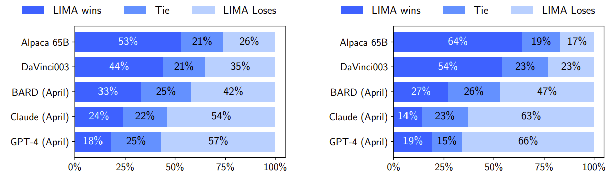
Figure on left presents results from our human preference study, while Figure on right shows GPT-4 preferences, with similar trends observed in both. Despite Alpaca 65B training on significantly more data, LIMA tends to produce more preferable outputs. DaVinci003, trained with RLHF, also falls short of LIMA’s performance. Bard occasionally outperforms LIMA but LIMA matches or exceeds Bard’s performance 58% of the time. Although Claude and GPT-4 generally perform better, LIMA occasionally produces superior responses, with even GPT-4 preferring LIMA outputs in 19% of cases.

Why Less is More ?

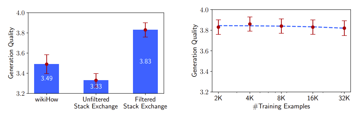
We investigate the effects of training data diversity, quality, and quantity through ablation experiments.We observe that, for the purpose of alignment, scaling up input diversity and output quality have measurable positive effects, while scaling up quantity alone might not

Experiment Setup: We fine-tune a 7B parameter LLaMa model on various datasets, maintaining consistent hyperparameters. Responses are graded for helpfulness on a likert scale by ChatGPT (GPT-3.5 Turbo), with results reported with confidence intervals.

Diversity: We compare Stack Exchange and wikiHow data to examine prompt diversity’s impact on response quality. Stack Exchange offers diverse prompts with excellent responses, while wikiHow presents homogeneous prompts. Training on Stack Exchange significantly outperforms wikiHow, indicating the importance of diversity.

Quality: We assess response quality by comparing models trained on Stack Exchange data with and without quality filters. The filtered dataset yields significantly better performance, highlighting the importance of response quality.

Quantity: Despite common wisdom suggesting increased training data improves performance, doubling the training set size from Stack Exchange does not enhance response quality. This finding suggests alignment’s scaling laws prioritize prompt diversity and high-quality responses over sheer quantity.

Task Generalization Capability

LIMA’s performance in multi-turn dialogue with just 1,000 single-turn interactions is assessed across 10 live conversations, with responses categorized as Fail, Pass, or Excellent. While responses demonstrate surprising coherence for a zero-shot chatbot, LIMA struggles to follow the prompt within 3 interactions in 6 out of 10 conversations.

To enhance LIMA’s conversational abilities, 30 multi-turn dialogue chains are collected, with 10 authored by the researchers and 20 derived from Stack Exchange comments. A new version of LIMA is fine-tuned using these examples, leading to significant improvements in generation quality. The proportion of excellent responses increases from 45.2% to 76.1%, while the failure rate drops noticeably. In addition, the fine-tuned model outperforms the zero-shot model in 7 out of 10 conversations, suggesting that limited supervision can invoke learned capabilities from pretraining.

The above is an example of a multi-turn dialogue case use to check task generalization capability.

Limitations and Conclusion

Fine-tuning a strong pretrained language model on 1,000 carefully curated examples can produce remarkable, competitive results on a wide range of prompts

Limitations: The mental effort in constructing such examples is significant and difficult to scale up. LIMA is not as robust as product-grade models while LIMA typically generates good responses, an unlucky sample during decoding or an adversarial prompt can often lead to a weak response

Paper 3: The Era of 1-bit LLMs: All Large Language Models are in 1.58 Bits

Introduction

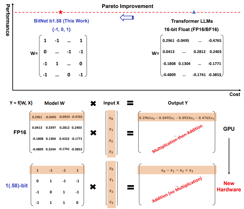
Large Language Models (LLMs) have seen significant growth in size and capabilities, leading to challenges in deployment and environmental concerns due to high energy consumption. Post-training quantization, reducing precision to create low-bit models for inference, has emerged as a solution. However, recent work on 1-bit model architectures like BitNet presents a promising direction for reducing LLM costs while maintaining performance. BitNet’s matrix multiplication involves only integer addition, saving energy costs and enabling faster computation.

In addition to computation, transferring model parameters during inference can be expensive. BitNet and its variant, BitNet b1.58, significantly reduce memory footprint and loading time from DRAM, leading to more efficient inference. BitNet b1.58 introduces an additional value of 0, offering stronger modeling capability by supporting feature filtering and matching full precision baselines in perplexity and end-task performance from a smaller size.

What is 1.58 bit ?

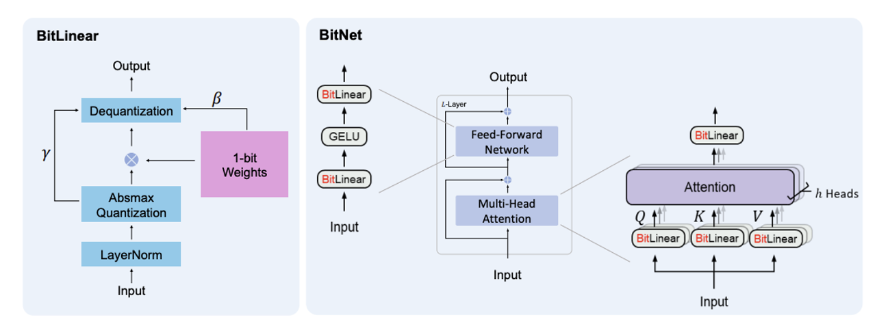
BitNet b1.58 is based on the BitNet architecture, which is a Transformer that replaces $\text{nn.Linear}$ with BitLinear. It is trained from scratch, with 1.58-bit weights and 8-bit activations. Compared to the original BitNet, it introduces some modifications that we summarize below.

Quantization Function. To constrain the weights to -1, 0, or +1, we adopt an absmean quantization function. It first scales the weight matrix by its average absolute value, and then round each value to the nearest integer among ${-1, 0, +1}$:

The quantization function for activations follows the same implementation in BitNet, except that we do not scale the activations before the non-linear functions to the range [0, $Q_b$]. Instead, the activations are all scaled to $[-Q_{b}, Q_{b}]$ per token to get rid of the zero-point quantization. This is more convenient and simple for both implementation and system-level optimization, while introduces negligible effects to the performance in our experiments.

Results

We compared BitNet b1.58 to our reproduced FP16 LLaMA LLM across various sizes, pre-training them on the RedPajama dataset for 100 billion tokens. Zero-shot performance was evaluated on tasks like ARC-Easy, ARC-Challenge, Hellaswag, Winogrande, PIQA, Open-bookQA, and BoolQ, alongside reporting validation perplexity on WikiText2 and C4 datasets. The runtime GPU memory and latency were also compared using FasterTransformer3, optimized for LLM inference latency on GPU devices. BitNet b1.58 matched full precision LLaMA LLM at 3B model size in perplexity, being 2.71 times faster and using 3.55 times less GPU memory. At 3.9B model size, BitNet b1.58 was 2.4 times faster, consumed 3.32 times less memory, and performed significantly better than LLaMA LLM 3B.

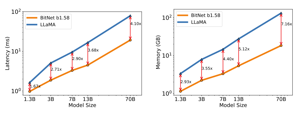
Decoding latency (Left) and memory consumption (Right) of BitNet b1.58 varying the model size.

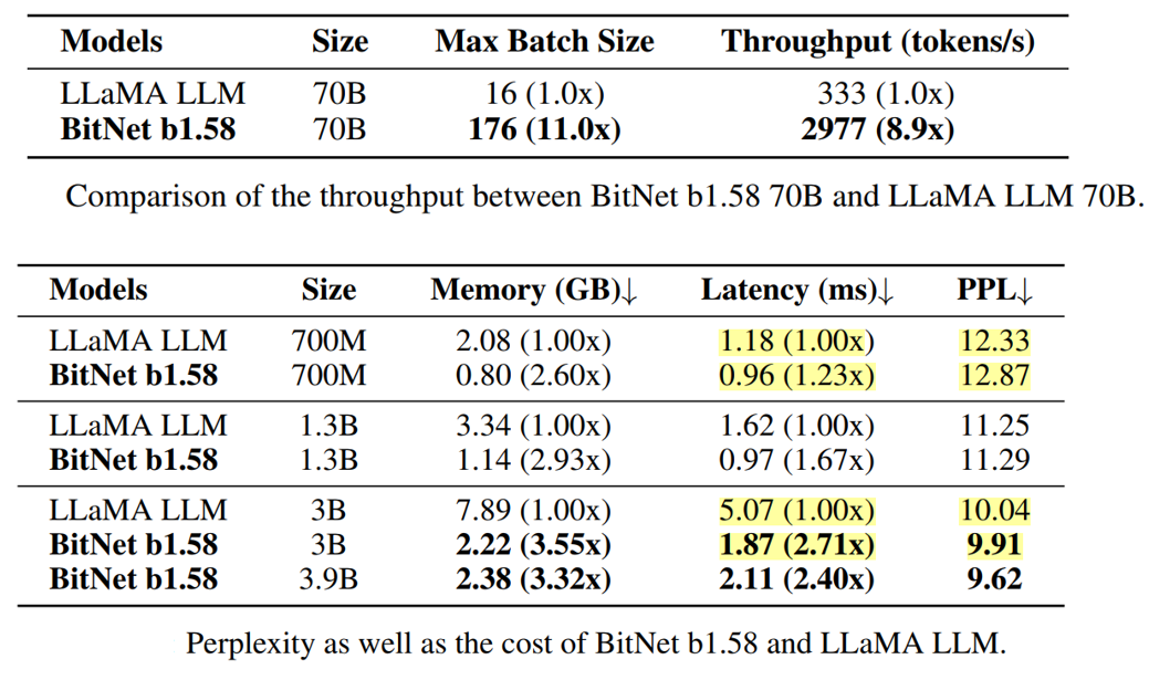
We scaled up the model size to 7B, 13B, and 70B and evaluated the cost. Figure above illustrates the trends of latency and memory, showing that the speed-up increases as the model size scales. In particular, BitNet b1.58 70B is 4.1 times faster than the LLaMA LLM baseline. This is due to the growing time cost for nn.Linear with the model size. The memory consumption follows a similar trend, as the embedding remains full precision and its memory proportion is smaller for larger models. Both latency and memory were measured with a 2-bit kernel, indicating potential for further optimization to reduce the cost )

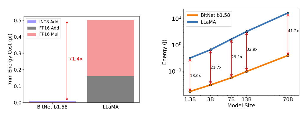
We estimate the energy consumption of arithmetic operations for both BitNet b1.58 and LLaMA LLM, focusing on matrix multiplication, which contributes most to LLM costs. Figure above shows the energy cost composition. BitNet b1.58 primarily involves INT8 addition calculations, while LLaMA LLM includes both FP16 addition and multiplication. Based on [Hor14, ZZL22], BitNet b1.58 saves 71.4 times energy consumption for matrix multiplication on 7nm chips. Additionally, we report end-to-end energy costs for models with 512 tokens. Our findings reveal that as model size increases, BitNet b1.58 becomes increasingly more energy-efficient compared to the FP16 LLaMA LLM baseline. This is attributed to nn.Linear’s growing percentage with model size, while costs from other components decrease for larger models.

Discussion and Conclusion

1-bit Mixture-of-Experts (MoE) LLMs offer a cost-effective solution by reducing computation FLOPs, addressing challenges of high memory consumption and inter-chip communication. The reduced memory footprint of 1.58-bit LLMs enables easier deployment of MoE models, reducing overhead in transferring activations across networks. BitNet b1.58 facilitates native support for long sequences by reducing activations from 16 bits to 8 bits, potentially doubling the context length with the same resources. This advancement can further be compressed to 4 bits or lower, enhancing long sequence handling capabilities. The use of 1.58-bit LLMs holds promise for improving language model performance on edge and mobile devices, overcoming limitations in memory and computational power. These devices can now deploy LLMs, expanding their application scope and enabling new functionalities. Additionally, 1.58-bit LLMs are well-suited for CPU devices commonly used in edge and mobile devices, enhancing their performance. Recent advancements in hardware like Groq demonstrate potential for building specific hardware for LLMs. There’s a call for designing new hardware optimized for 1-bit LLMs, leveraging the unique computation paradigm enabled by BitNet.