Advanced Transformer Architectures

• SlideDeck: W14_LLM_advanced_arch
• Version: current
• Lead team: team-6
• Blog team: team-6

Efficiency

In this session, our readings cover:

Required Readings:

Advancing Transformer Architecture in Long-Context Large Language Models: A Comprehensive Survey

• https://arxiv.org/abs/2311.12351
• Transformer-based Large Language Models (LLMs) have been applied in diverse areas such as knowledge bases, human interfaces, and dynamic agents, and marking a stride towards achieving Artificial General Intelligence (AGI). However, current LLMs are predominantly pretrained on short text snippets, which compromises their effectiveness in processing the long-context prompts that are frequently encountered in practical scenarios. This article offers a comprehensive survey of the recent advancement in Transformer-based LLM architectures aimed at enhancing the long-context capabilities of LLMs throughout the entire model lifecycle, from pre-training through to inference. We first delineate and analyze the problems of handling long-context input and output with the current Transformer-based models. We then provide a taxonomy and the landscape of upgrades on Transformer architecture to solve these problems. Afterwards, we provide an investigation on wildly used evaluation necessities tailored for long-context LLMs, including datasets, metrics, and baseline models, as well as optimization toolkits such as libraries, frameworks, and compilers to boost the efficacy of LLMs across different stages in runtime. Finally, we discuss the challenges and potential avenues for future research. A curated repository of relevant literature, continuously updated, is available at this https URL.

FlashAttention: Fast and Memory-Efficient Exact Attention with IO-Awareness

• Tri Dao, Daniel Y. Fu, Stefano Ermon, Atri Rudra, Christopher Ré
• Paper: https://arxiv.org/abs/2205.14135

• Transformers are slow and memory-hungry on long sequences, since the time and memory complexity of self-attention are quadratic in sequence length. Approximate attention methods have attempted to address this problem by trading off model quality to reduce the compute complexity, but often do not achieve wall-clock speedup. We argue that a missing principle is making attention algorithms IO-aware – accounting for reads and writes between levels of GPU memory. We propose FlashAttention, an IO-aware exact attention algorithm that uses tiling to reduce the number of memory reads/writes between GPU high bandwidth memory (HBM) and GPU on-chip SRAM. We analyze the IO complexity of FlashAttention, showing that it requires fewer HBM accesses than standard attention, and is optimal for a range of SRAM sizes. We also extend FlashAttention to block-sparse attention, yielding an approximate attention algorithm that is faster than any existing approximate attention method. FlashAttention trains Transformers faster than existing baselines: 15% end-to-end wall-clock speedup on BERT-large (seq. length 512) compared to the MLPerf 1.1 training speed record, 3$\times$ speedup on GPT-2 (seq. length 1K), and 2.4$\times$ speedup on long-range arena (seq. length 1K-4K). FlashAttention and block-sparse FlashAttention enable longer context in Transformers, yielding higher quality models (0.7 better perplexity on GPT-2 and 6.4 points of lift on long-document classification) and entirely new capabilities: the first Transformers to achieve better-than-chance performance on the Path-X challenge (seq. length 16K, 61.4% accuracy) and Path-256 (seq. length 64K, 63.1% accuracy).

• Related: blogpost FlashAttention — Techniques for Efficient Inference of LLMs (III/IV)

JAMBA

• Introducing Jamba: AI21’s Groundbreaking SSM-Transformer Model Debuting the first production-grade Mamba-based model delivering best-in-class quality and performance.
• March 28, 2024
• https://www.ai21.com/blog/announcing-jamba
• We are thrilled to announce Jamba, the world’s first production-grade Mamba based model. By enhancing Mamba Structured State Space model (SSM) technology with elements of the traditional Transformer architecture, Jamba compensates for the inherent limitations of a pure SSM model. Offering a 256K context window, it is already demonstrating remarkable gains in throughput and efficiency—just the beginning of what can be possible with this innovative hybrid architecture. Notably, Jamba outperforms or matches other state-of-the-art models in its size class on a wide range of benchmarks.

More readings:

Mamba: Linear-Time Sequence Modeling with Selective State Spaces

• Albert Gu, Tri Dao
• https://arxiv.org/abs/2312.00752
• Foundation models, now powering most of the exciting applications in deep learning, are almost universally based on the Transformer architecture and its core attention module. Many subquadratic-time architectures such as linear attention, gated convolution and recurrent models, and structured state space models (SSMs) have been developed to address Transformers’ computational inefficiency on long sequences, but they have not performed as well as attention on important modalities such as language. We identify that a key weakness of such models is their inability to perform content-based reasoning, and make several improvements. First, simply letting the SSM parameters be functions of the input addresses their weakness with discrete modalities, allowing the model to selectively propagate or forget information along the sequence length dimension depending on the current token. Second, even though this change prevents the use of efficient convolutions, we design a hardware-aware parallel algorithm in recurrent mode. We integrate these selective SSMs into a simplified end-to-end neural network architecture without attention or even MLP blocks (Mamba). Mamba enjoys fast inference (5× higher throughput than Transformers) and linear scaling in sequence length, and its performance improves on real data up to million-length sequences. As a general sequence model backbone, Mamba achieves state-of-the-art performance across several modalities such as language, audio, and genomics. On language modeling, our Mamba-3B model outperforms Transformers of the same size and matches Transformers twice its size, both in pretraining and downstream evaluation.

Efficient Memory Management for Large Language Model Serving with PagedAttention

• Woosuk Kwon, Zhuohan Li, Siyuan Zhuang, Ying Sheng, Lianmin Zheng, Cody Hao Yu, Joseph E. Gonzalez, Hao Zhang, Ion Stoica
• High throughput serving of large language models (LLMs) requires batching sufficiently many requests at a time. However, existing systems struggle because the key-value cache (KV cache) memory for each request is huge and grows and shrinks dynamically. When managed inefficiently, this memory can be significantly wasted by fragmentation and redundant duplication, limiting the batch size. To address this problem, we propose PagedAttention, an attention algorithm inspired by the classical virtual memory and paging techniques in operating systems. On top of it, we build vLLM, an LLM serving system that achieves (1) near-zero waste in KV cache memory and (2) flexible sharing of KV cache within and across requests to further reduce memory usage. Our evaluations show that vLLM improves the throughput of popular LLMs by 2-4× with the same level of latency compared to the state-of-the-art systems, such as FasterTransformer and Orca. The improvement is more pronounced with longer sequences, larger models, and more complex decoding algorithms. vLLM’s source code is publicly available at this https URL

Attention Mechanisms in Computer Vision: A Survey

• Meng-Hao Guo, Tian-Xing Xu, Jiang-Jiang Liu, Zheng-Ning Liu, Peng-Tao Jiang, Tai-Jiang Mu, Song-Hai Zhang, Ralph R. Martin, Ming-Ming Cheng, Shi-Min Hu
• https://arxiv.org/abs/2111.07624
• Humans can naturally and effectively find salient regions in complex scenes. Motivated by this observation, attention mechanisms were introduced into computer vision with the aim of imitating this aspect of the human visual system. Such an attention mechanism can be regarded as a dynamic weight adjustment process based on features of the input image. Attention mechanisms have achieved great success in many visual tasks, including image classification, object detection, semantic segmentation, video understanding, image generation, 3D vision, multi-modal tasks and self-supervised learning. In this survey, we provide a comprehensive review of various attention mechanisms in computer vision and categorize them according to approach, such as channel attention, spatial attention, temporal attention and branch attention; a related repository this https URL is dedicated to collecting related work. We also suggest future directions for attention mechanism research.

State Space Model for New-Generation Network Alternative to Transformers: A Survey

Motivation

Pros and Cons of Attention

• Self-attention mechanism has successfully enabled transformer to learn long-range feature representations well.
• However, Transformer-based models require high-end GPU with larger memory for training and testing/deployment.

Hence, We need a model that not only requires less computing cost but also is still able to capture long-range dependencies while maintaining high performance.

That’s what State Space Model (SSM) wants to solve.

Formulation of SSM

SSM is a commonly used model in control theory and is used in Kalman simulation and hidden Markov models. Its basic formulation is shown in the figure below.

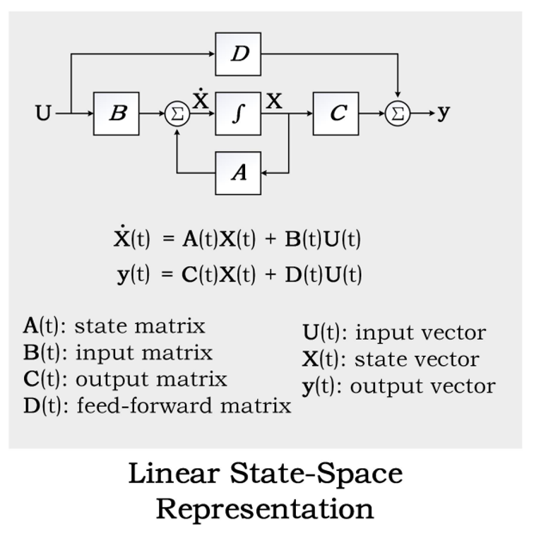
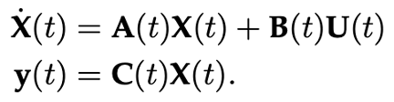
Normally, we would omit the parameter D (assume D=0 becuase the term Du can be viewed as a skip connection and is easy to compute). So a more common formulation we would see in most state space model would be as:

Discretization

As a continuous system, it is hard for SSM to be used in modern deep learning algorithm. In practice, we always deal with discrete data, such as text. This requires us to discretize the SSM, transforming our continuous parameters A, B, C into discrete parameters $\hat{A}, \hat{B}$ using zero-order hold rule (ZOH) as shown in Figure below. Readers can refer to the paper for detailed derivation.

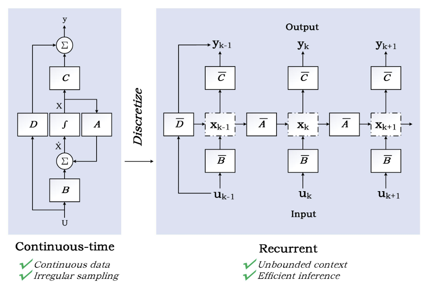
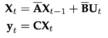
In conclusion, the discretized version of SSM is like:

Convolutional Form

Unlike RNN, SSM here doesn’t have non-linear functions. So we can try to expand $y_t$ and surprisingly find SSM can be written in convolutional form.

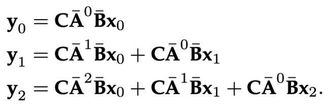
Looking at the result of the expansion above, we can see that the coefficient of each $x_t$ can be extracted out and write a convolutional kernel:

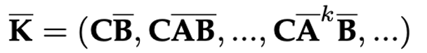
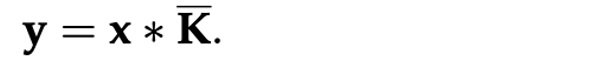
Hence, we can write our SSM formulation as:

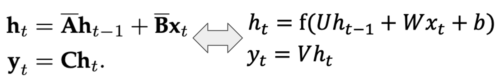
It’s easy to find that SSM is very similar to RNN. Comparing the formulation of SSM and RNN below, we can find the main reason why RNN can’t be written in convolutional form and thus can’t be trained efficiently is the non-linear funciton $f$.

Structured State Space Model (S4)

• Similar to RNNs, SSM also suffers from the vanishing/exploding gradients problem when modeling longer sequences.

To solve this problem, HiPPO matrices is introduced which combines the concepts of Recurrent Memory and Optimal Polynomial Projections, thus can significantly improve the performance of recursive memory.

In practice, we would use HiPPO matrix to initial like matrix A.

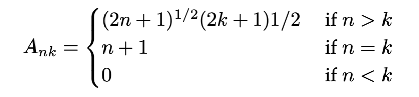
Note the “Structured” comes from the HiPPO matrix. And we usually can the vallila SSM with HiPPO matrix :S4 model in short which will be seen in most SSM related papers.

From S4 to Mamba (S6)

The problem of S4:

• S4 does not have selectivity
• Those discrete parameters are constant Those problem will result in the S4 treat all part of the input exactly the same like the Figure shown below.

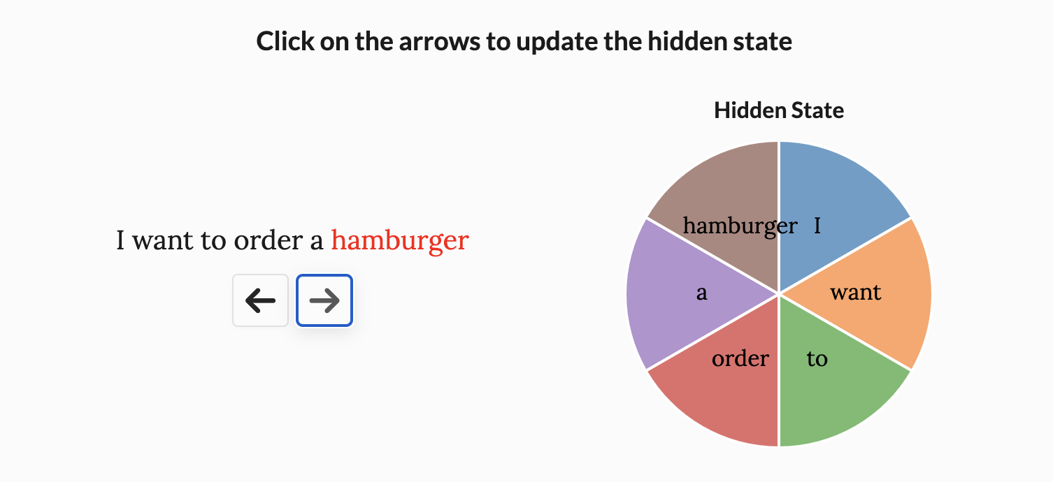
Mamba makes these parameters vary based on the input, like the formulation below:

By doing so, model has the ability to focus on certain words, like the Figure shown below.

Parallization of Mamba

• In S4, we are able to precompute this kernel, save it, and multiply it with the input x.
• However, in Mamba, these matrices change depending on the input.
• If we want selectivity, we’ll need to train Mamba with RNN mode.

Mamba is able to solve this problem through parallel scan.

Parallel Scan Whether an operation can be done in parallel depends on associative property. Mamba’s recurrence was very similar to a scan algorithm, also known as a prefix sum.

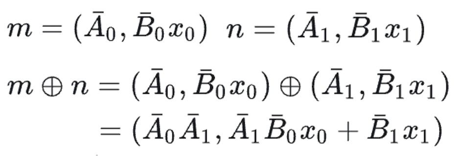
We can verify its associative property with a new variable k:

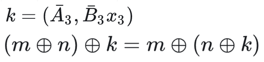
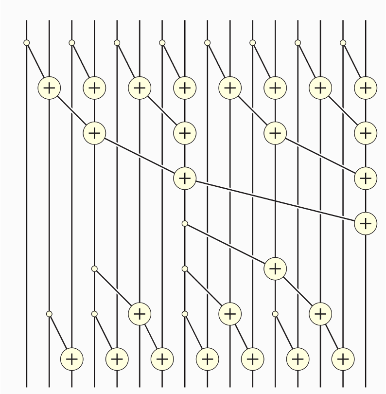
Figure below shows how parallel scan works. We can pick any vertical line and start from the top of this line and move to the bottom, tracing each addition back to the array’s first few items. By the time we reach the bottom, we should have the sum of all items to the left of this line.

Variations of SSM

Language Modeling

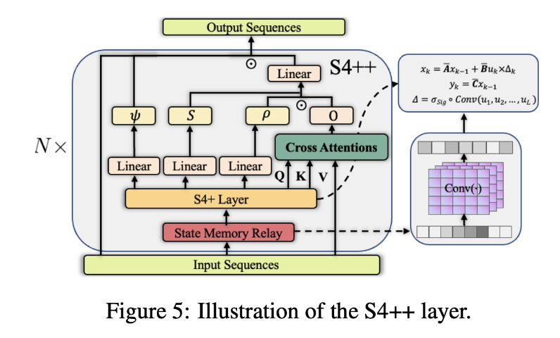
S4+++: -State Memory Relay. -Integrate complex dependency bias via an interactive cross-validation mechanism.

Voice Task

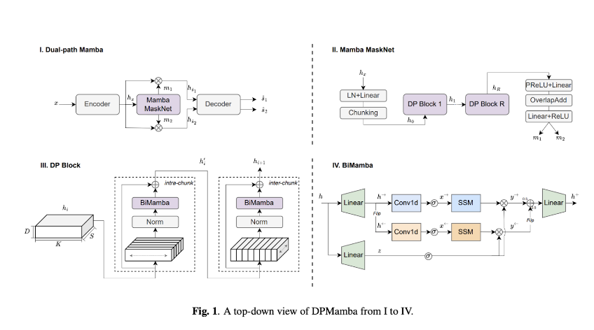
DP-Mamba -Bidirectional Dependency Modeling: Simultaneously models both short-term and long-term forward and backward dependencies of speech signals. -Selective State Space: Enhances model capability through a selectively utilized state space. -Performance: Achieves comparable results to the dual-path Transformer model Sepformer.

SP-Mamba:

• Utilizes TF-GridNet.
• Replaces the Transformer module with a bidirectional Mamba module.
• Result: Captures a wider range of language information, leading to broader comprehension.

Variations in Computer Vision

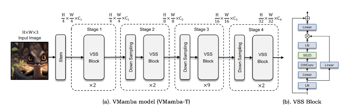
VMamba VMamba uses linear complexity to capture the full range of sensory fields, introduces traversal of spatial information across scan blocks, and converts non-causal visual images into ordered patch sequences.

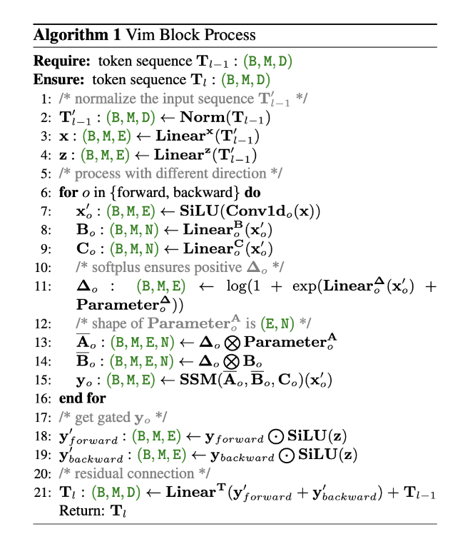
Vision Mamba

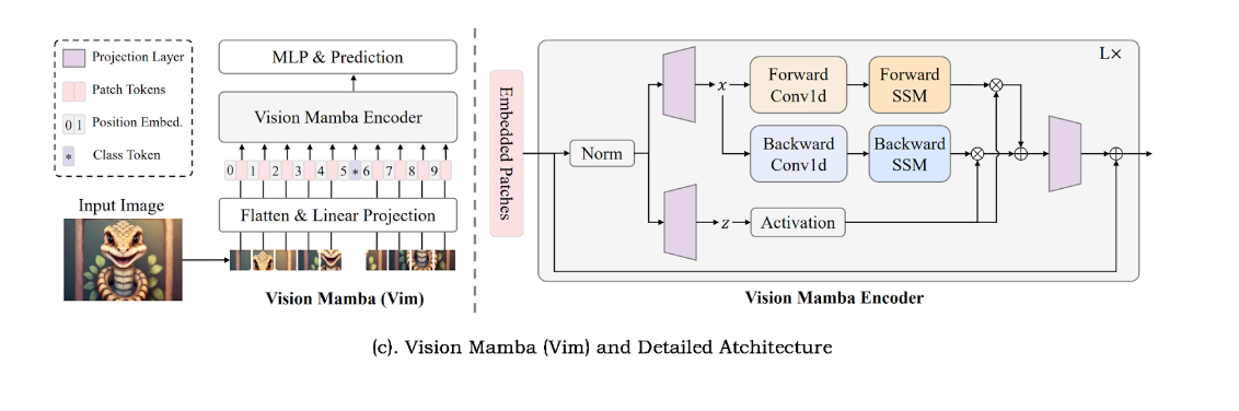
The Vim model divides the input image into chunks and then projects the chunks into tokens at the begining. These tokens are then fed into the Vim encoder. For tasks like ImageNet classification, an additional learnable classification token is added to the sequence of token labels (this labels are used consistently in this way from the beginning of heavy BERT). Unlike the Mamba model used for modeling text sequences, the Vim encoder processes the token sequence in both the forward and reverse directions.

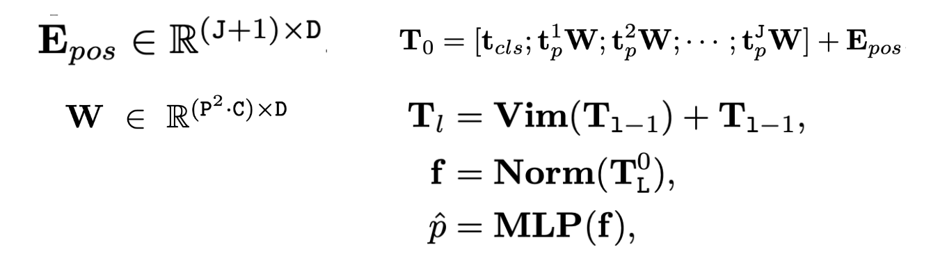
And the Vim encoder will be shown in the figure below

Mamba Variations in different Task

• Classification task: Vim VMamba
• Detection task: MiM-ISTD
• Segmentation task
• Medical image segmentation: VM-UNet
• Medical tasks
• Registration task: MambaMorph
• Restoration task: MambdaIR
• Generation task: ZigMa
• Video understanding:ViS4mer, Video Mamba

Variations in Graph

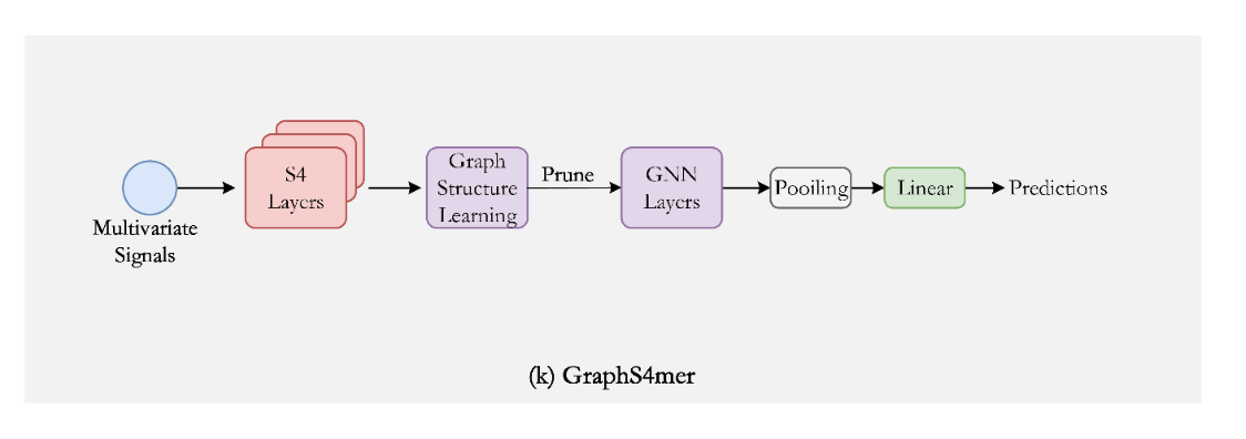
GraphS4mer: Using the S4 architecture to capture long-range dependencies and includes a dynamic graph structure learning layer for spatial correlations.

GMN: Based on selective State Space Models, tackling the limitations of traditional GNNs in capturing long-range dependencies and computational efficiency.

Variations in Multi-modality and Multi-media

• S4ND Model:
  • Extends State Space Models to multidimensional signals.
  • Effective in large-scale visual data modeling across 1D, 2D, and 3D dimensions.
  • Proven applications in image and video classification.
• VL-Mamba:
  • First implementation of the state-space model Mamba in multimodal tasks.
  • Aims to address high computational costs in Transformer architectures.
• CMViM:
  • Focuses on multimodal learning for 3D high-resolution medical images, specifically Alzheimer’s disease.
  • Utilizes the MAE framework, replacing the ViT module with a simpler Vim module to reduce computational complexity from quadratic to linear.
  • Enhances modeling capabilities through intra-modality and inter-modality contrastive learning, improving feature discrimination and aligning representations across different modalities.

Variation for Time Serires

TimeMachine Purpose: Addresses challenges in long-term time-series forecasting (LTSF). Key Challenges:

• Capturing long-term dependency relationships.
• Overcoming poor linear scalability in time-series data. Innovative Solution:
• Uses multiple Mamba modules integrated into a singular architecture to enhance dependency capture and improve channel mixing.
• Provides selective prediction capabilities for both global and local contexts across various scales.
• Results: Demonstrated significant improvements in accuracy and scalability in experimental validations.

Advancing Transformer Architecture in Long-Context Large Language Models: A Comprehensive Survey

Introduction to Long-Context LLMs

• Great Success for Transformer-based LLM Models (chatGPT, Bert, Claude..)

  • Indicates a potential path towards AGI
  • Revolutionizing Application: Document summarization, Computer vision, …
  • Essential for advanced applications
    • like detailed text analysis and interactive AI systems

• Success due to well-designed Attention Mechanism, but …

Challenges and Research Directions in Long-Context LLMs

• Challenges in Current Transformer Models

  • Complexities: High computational needs with quadratic time and space complexities during training and inference
    • Performance Degradation: Lack of robustness in mechanism leads to performance degradation with long sequences

• Research Directions

  • Efficiency Improvements: Attention mechanism, memory mechanisms
  • Handling Long Contexts: Effective length generalization, context pre/post processing

Contributions of this Survey

• Holistic Taxonomy:Detailed breakdown of Transformer architecture enhancements
• Evaluations and Toolkits: Analysis of datasets, metrics, libraries, frameworks for optimizing LLM efficiency
• Future Directions: Identifying key challenges and potential solutions for advancing long-context comprehension in LLMs.

Section 2: Overview

Preliminaries of Neural Language Modeling

• Modeling Stages
  • Preprocessing: Tokenization of raw text into subwords or tokens
  • Pretraining: Learning semantic patterns and linguistic structures on large corpora
  • Fine-tuning: Adapting the pre-trained model to task-specific data for downstream applications
  • Inference: Auto regressively generating text based on learned probabilities
• Key-Value Cache in LLMs
  • Functionality: Stores key-value pairs for attention, extending sequences during generation
  • Limitation: Linearly growing memory occupation with generated tokens, prompting long-term memory enhancements

Limitations of Transformer Architecture in Handling Long Contexts

• Attention Complexity
  • Computational Complexity: In scenarios where sequence length 𝐿 far exceeds dimension 𝑑
    • The complexity becomes quadratic
    • Time Complexity: 𝑂(𝐿^2*d) Space Complexity: 𝑂(𝐿^2)
• In-context Memory Limitations
  • Statelessness of Transformers: Lacks a mechanism to retain state between calls, relying only on the KV cache
  • Impact on Applications: This design limits effectiveness in applications requiring long-term memory(chatbots)
• Max-Length Constraint
  • Training and Inference: Engineers set a maximum sequence length 𝐿𝑚𝑎𝑥 to prevent memory overflow
    • As a hyper-parameter, typically between 1K, 2K 4K tokens
  • Performance degradation: observed when handling inputs longer than 𝐿𝑚𝑎𝑥 resulting in implausible outputs

Roadmap of Enhancements for Long-Context Capabilities in LLMs

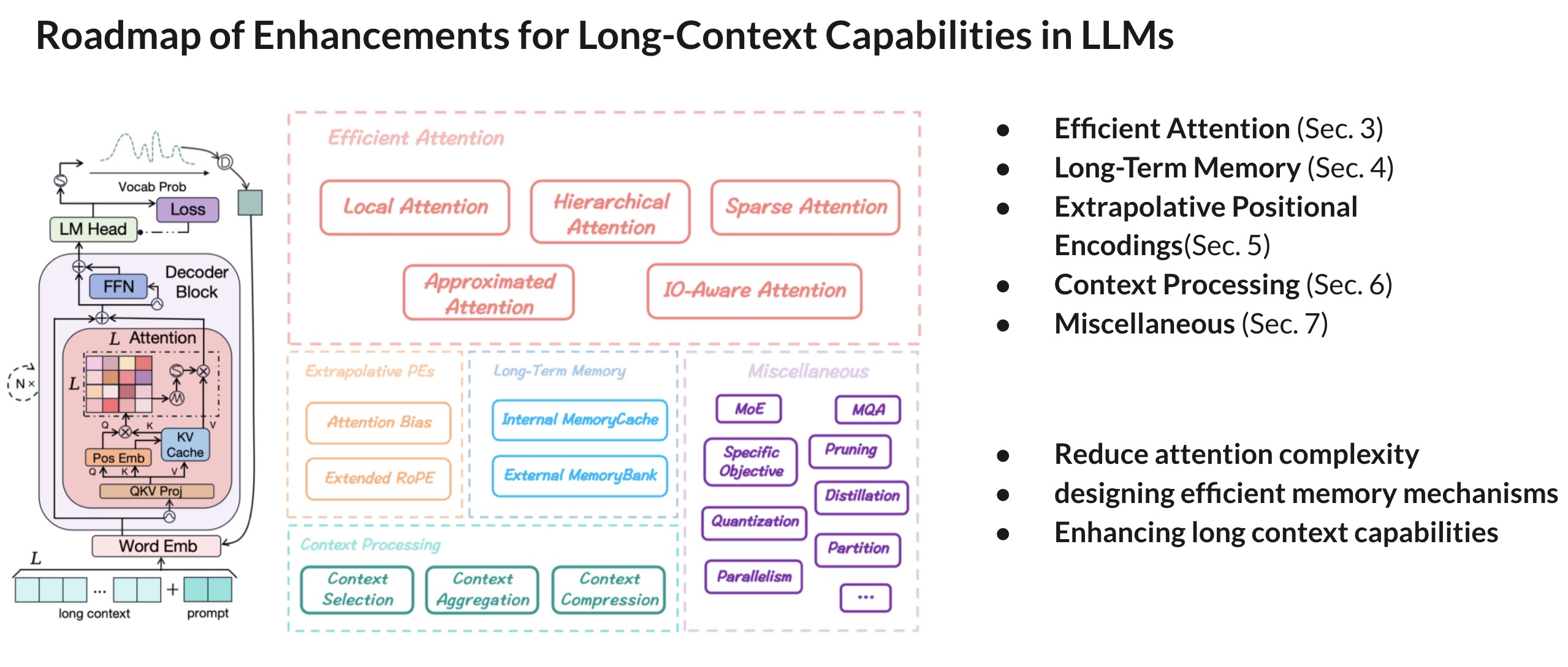
Section 3: Efficient Attention Mechanisms

• Goal: Addressing the computational bottleneck of attention mechanisms in Transformers
• Impact: Expanding the context length boundary for LLMs during both pre training and inference phases
• Category
  • Local Attention
  • Hierarchical Attention
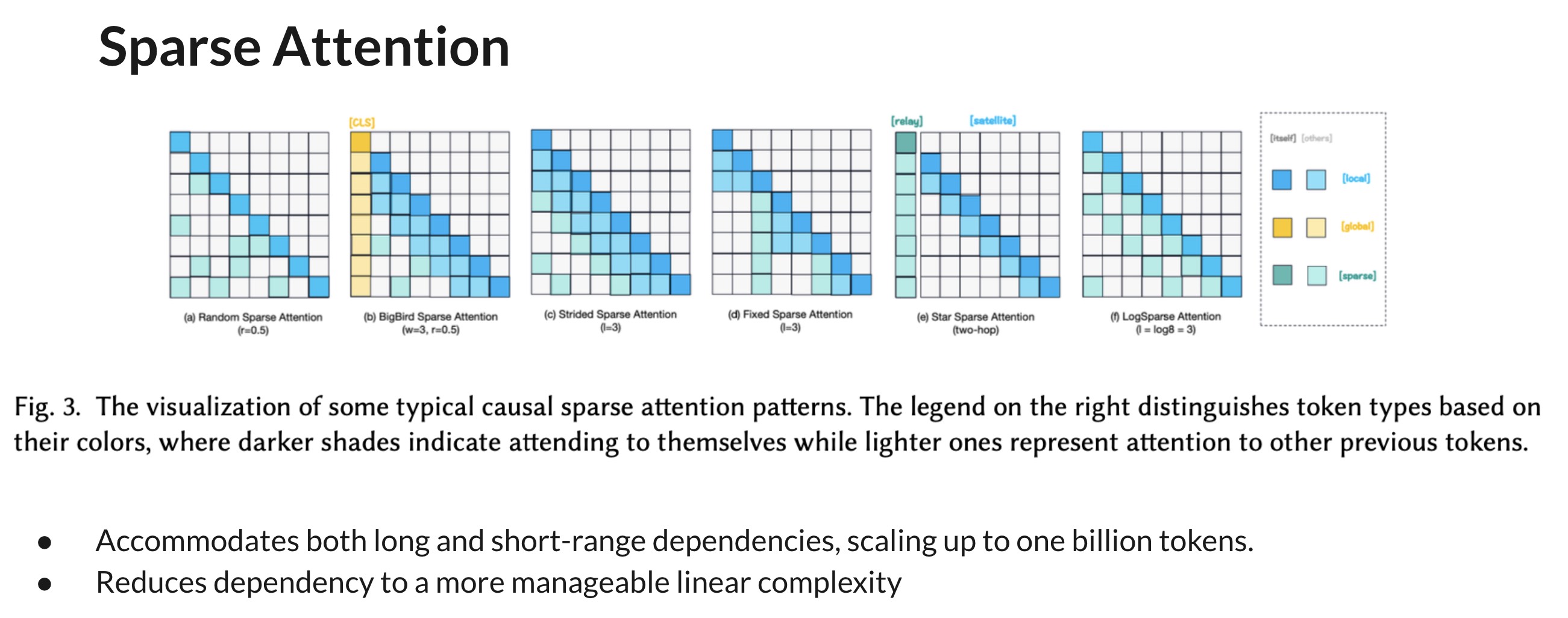
  • Sparse Attention
  • Approximated Attention
  • IO-Aware Attention

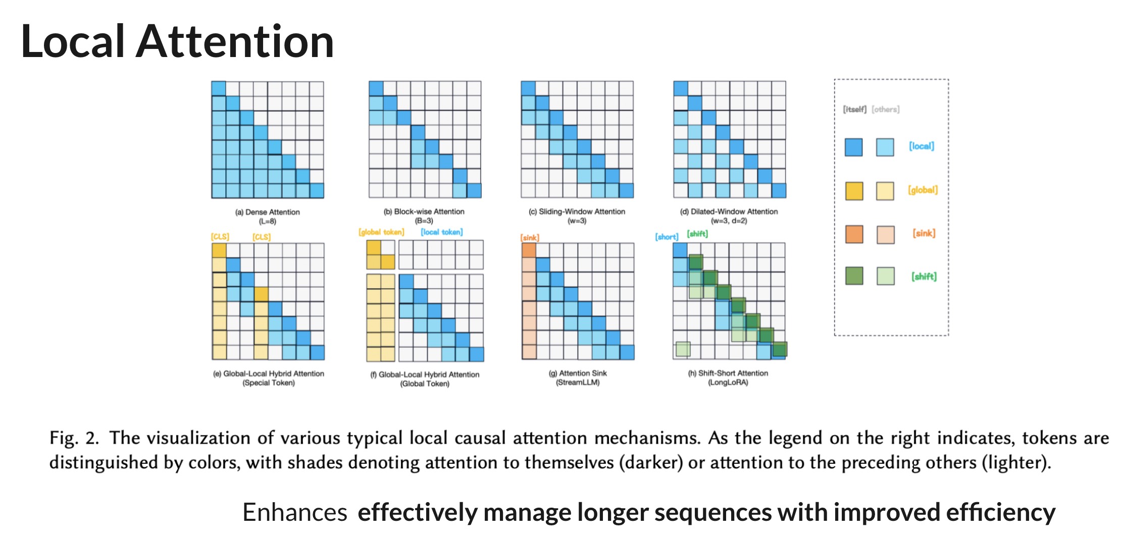
Local Attention

• Redefining Attention Mechanisms
  • Traditional Global Attention: Each token attends to all others, leading to 𝑂(𝐿^2𝑑) complexities
  • Local Attention: Focuses on neighboring tokens, reducing time and space complexities
• Approaches
  • Block-wise Attention
    • Divides input into non-overlapping blocks, each attending within itself(e.g. BlockBERT)
  • Sliding Window Attention
    • Each token attends within a fixed-size window, inspired by CNN techniques(e.g. Longformer)
  • Global-Local Hybrid Attention
    • Combines local attention with global tokens for broader context (e.g. LongLM)
  • LSH Attention
    • Utilizes locality-sensitive hashing for efficient neighbor token selection

Hierarchical Attention

• Goal: Merge higher-level global information with lower-level local attention for efficient and scalable processing
• Impact
  • Complexity Reduction: Achieves sub-quadratic computational and memory costs while preserving the expressiveness of full attention
  • Contextual Balance: Maintains a balance between local and global context for inherent locality principle
• Approaches
  • Two-Level Hierarchy
    • Uses self-attention across two levels: word-to-sentence and sentence-to-document (e.g. HAN)
  • Multi-Level Hierarchy
    • **Introduces fine-to-coarse attention via **binary partitioning**, formalizing as a graph neural network(e.g BPT)
    • Controls attention span with a soft attention mask (e.g. Adaptive Span Transformer)
  • Advanced Hierarchical Mechanisms
    • Partitions attention matrix into blocks with different low-rank ranges (e.g. H-Transformer-1D)
    • Combines full-attention approximation with structured factorization (e.g. Combiner)

Approximated Attention

• Goal: Reduce the full attention computation by leveraging sparsity and low-rankness with linear complexity, optimizing precision trade-offs
• Impact: Provides sub-quadratic computation and memory complexity while maintaining the expressiveness of full attention
• Techniques
  • Low-Rank Approximation
    • Linformer: Utilizes SVD for a low-rank approximation of the attention matrix, reducing complexity to 𝑂(𝐿𝑘𝑑)
  • Nested Attention
    • Luna: Combines pack and unpack attention strategies to handle sequences of varying lengths without compromising parallelism
  • Kernelized Approximation
    • Linear Transformer & Performer: Introduces kernel-based attention approximations, significantly cutting down on computational resources
  • Hybrid Approaches
    • Sparse-Kernelized Hybrid
    • Scatterbrain: combines sparse matrices and kernelized feature maps for enhanced efficiency and precision

IO-Aware Attention

• Different
  • Previous attention methods trade off some attention quality for lower computation
  • But IO-aware methods maintain exactness of attention calculations while optimizing computational resources
• Offer exact attention computations with significantly reduced memory and time consumptionA leap forward in the optimization of Transformer models for large-scale applications
• Techniques
  • Memory-Efficient Attention: Utilizes lazy softmax algorithm for numerically stable attention
  • Flash Attention: Achieves up to 7.6x speedup and 20x memory efficiency with exact attention computation
  • Paged AttentionAddresses inference memory bottlenecks by managing KV cache memory with virtual memory paging techniques, improving efficiency and flexibility for batched requests
  • Innovations and ImprovementsSparse Clustered Factorization Attention: Extends Flash Attention to accommodate diverse sparsity patterns, leading to 2 to 3.3 times training speedup
  • Virtual Large Language Models: Proposes techniques to manage growing KV cache memory

Section 4: Long-Term Memory

Because of in-context working memory, the Transformer architecture often struggles with capturing long-term dependencies. The researchers propose two main avenues to address this challenge: (1) Internal MemoryCache; (2) External MemoryBank.

Section 4: Long-Term Memory

Internal MemoryCache

For Internal MemoryCache, there are different types:

• Segment-Level Recurrence.
  • It caches the output of 𝑚 previous consecutive segments in the last layer and concatenates them into the current segment in the present layer to extend the context for the current query.
• Retrospective Recurrence.
  • It concatenates the output hidden states of previous segments in the same layer, instead of the last layer.
• Continuous-Signal Memory.
  • The ∞-former model uses a continuous signal representation to achieve unbounded long-term memory.

External MemoryBank

For External MemoryBank, there are different types:

• Cosine-Based Retrieval Criteria.
  • LangChain is an open-source framework designed for chatbots, which processes local documentation into a memory bank using LLMs and retrieves context using cosine similarity to enhance interaction and response generation.
• Heuristic Retrieval Criteria.
  • It’s used for enhancing large language models with memory banks, enabling more efficient and context-aware data handling and retrieval in applications like chatbots and knowledge-based systems.
• Learnable Retrieval Criteria.
  • REALM use MLM to train a neural knowledge retriever
  • LongMem decouples the memory retrieval process using a SideNet.
  • FOT introduces a novel contrast training method to refine the key-value space and enhance retrieval accuracy as the size of the memory bank expands.

In summary, Internal MemoryCache trades space for time by using caching mechanisms to reduce computation. However, after model training is completed, it is difficult to update the internal knowledge, which is why such methods are rarely used nowadays. Instead, the External Memory Bank method is mainly used.

Section 5: Extrapolative PEs

The meaning of PEs is Extrapolative Positional Encodings. Current PEs play the undeniable role in length generalization in more general scenarios.

• Enhancing Understanding
  • Rethinking PEs as 𝛽-Encoding.
  • Length Extrapolation Dilemma.
• Attention Bias
  • As alternative mechanisms to explicitly encoding positional information, attention bias have been explored to capture the sequentiality and temporality of natural language incorporated into the attention kernel.
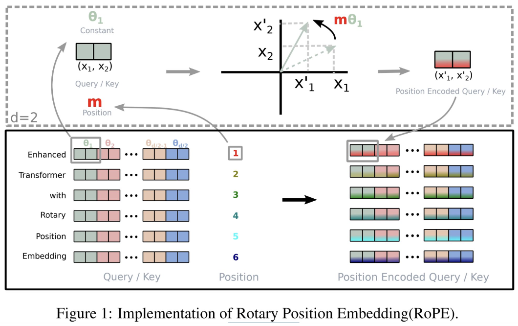
• Extended RoPE
  • Several research works have aimed to extend RoPE using various strategies to enhance its length extrapolation capabilities, including Scaling Strategies, Truncation Strategies, and Rearrangement Strategies.

Section 6: Context Processing

There are three different strategies:

• Context Selection
  • Various strategies employed by different models to effectively manage long text segments within the limited context window of LLMs, involving segment partitioning, scoring based on selection criteria, and iterative or simultaneous selection processes to prioritize the most relevant segments for processing.
• Context Aggregation
  • Extracting and integrating information from all context segments to generate a coherent final answer, through techniques like Fusion-in-Decoder, Map Reduce, Refinement.
  • Handling parallel context windows, each with different strategies for encoding, merging, and refining the information from multiple segments.
• Context Compression
  • Methods for compressing long contexts to fit within the maximum sequence length constraints of LLMs.
    • Soft compression: create condensed and abstract representations through embedded learning.
    • Hard Compression: eliminate redundancies using metrics like self-information and perplexity to optimize input quality before processing.

Section 7: Miscellaneous Solution

The miscellaneous solution talked in the part are not be exhaustive or specific to Transformer-based models. Many of these techniques are applicable universally to any model equipped with deep neural networks, albeit particularly crucial for large-scale LLMs. Some solutions are as follows:

• Specific Objectives
  • Recent research explores tailored approaches to adapt pretraining for specific tasks, aiming to enhance LLMs’ effectiveness in capturing intricate long-range dependencies and discourse structures in longer texts compared to shorter ones. (XLNet, ERNIE-Doc, DANCE, PEGASUS, PRIMERA)
• Mixture of Experts
  • Mixture of Experts (MoE) enhances large language models by incorporating specialized expert modules and dynamic gating mechanisms to optimize task performance, reduce computational demands, and improve efficiency and effectiveness in handling large-scale contexts.
• Parallelism
  • Leveraging modern aggregated GPU memory within and across nodes, recent research has introduced various parallelism strategies to scale up model sizes and extend sequence length, including Data Parallelism (DP), Tensor Parallelism (TP), Pipeline Parallelism (PP), Sequence Parallelism (SP), Expert Parallelism (EP).
• Weight Compression
  • Various methods enhance memory efficiency in large-scale LLMs through weight compression techniques, including pruning, factorization, quantization, partitioning, and distillation.

Section 8: Evaluation Necessity & Optimization Toolkit

The researchers explore evaluation necessities for assessing long-context capabilities of LLMs, including datasets, metrics, and baseline models. And they investigate popular optimization toolkits, such as libraries, frameworks, and compilers, to enhance LLM efficiency and effectiveness during development.

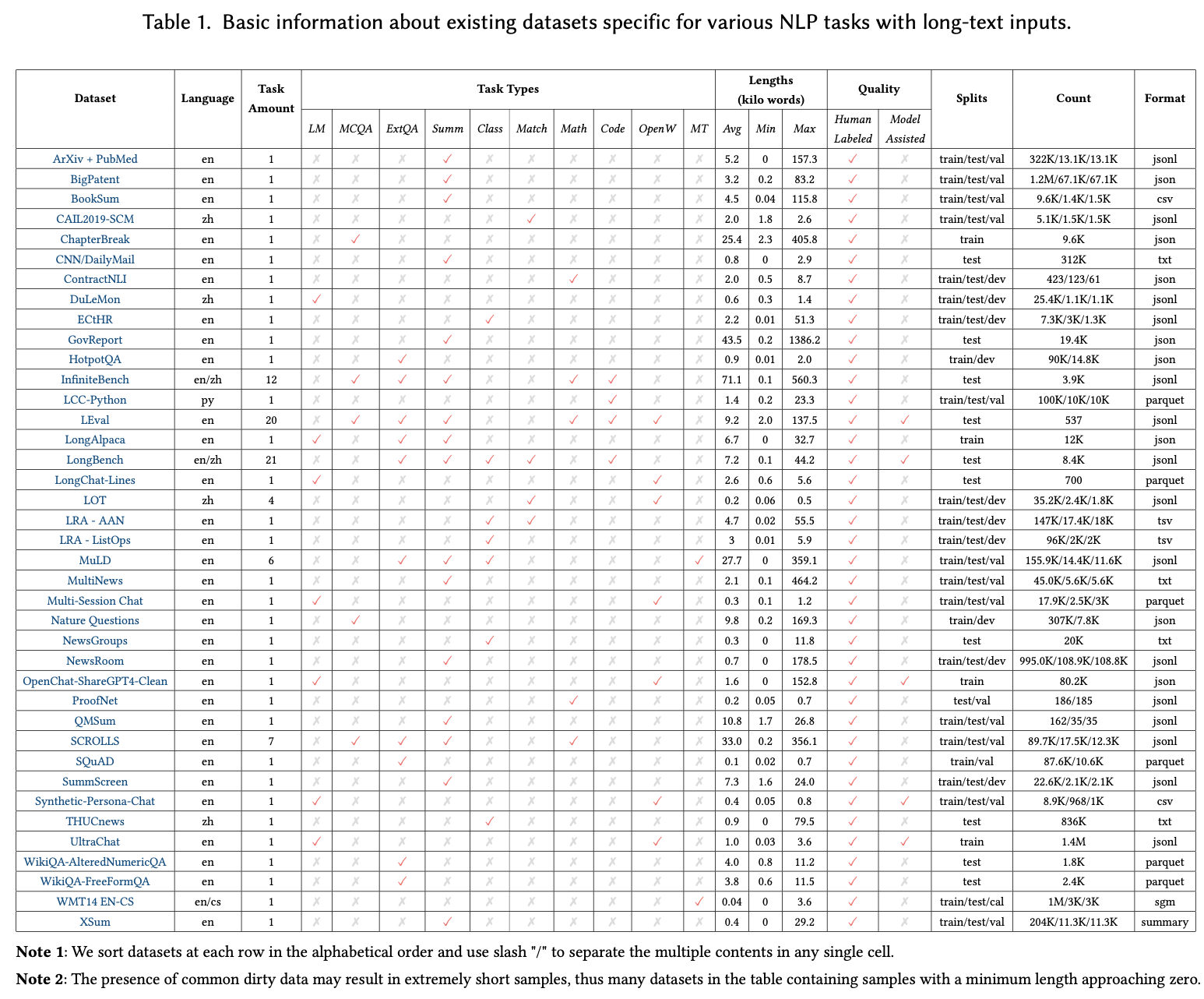
For Datasets, detailed information on each dataset is available in Table 1, covering language, task types, length statistics, quality, splits, count and format.

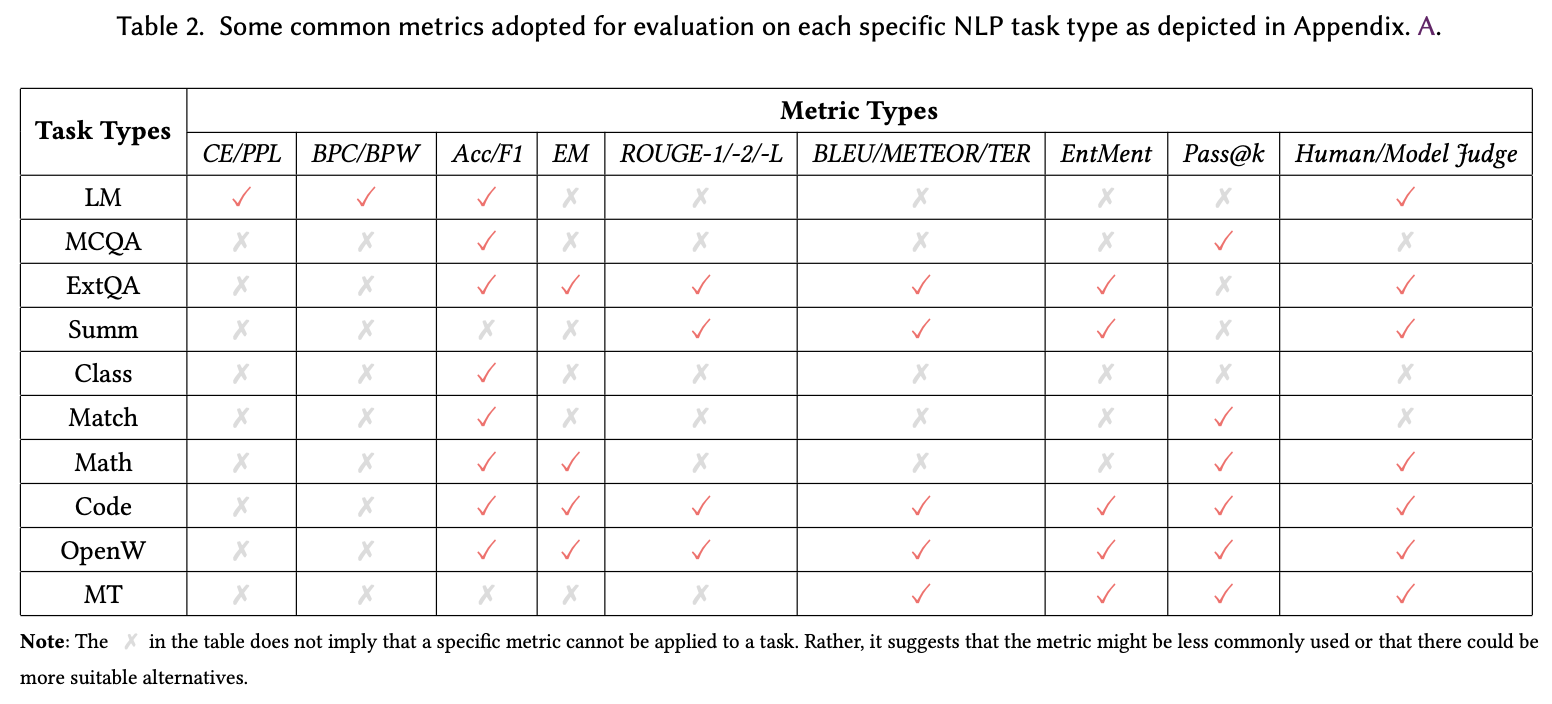
For Metrics, Table 2 provides a summary of nine categories of general evaluation metrics commonly employed across ten NLP task types, encompassing language modeling, question answering, summarization, math solving, code generation, and open-ended writing, among others.

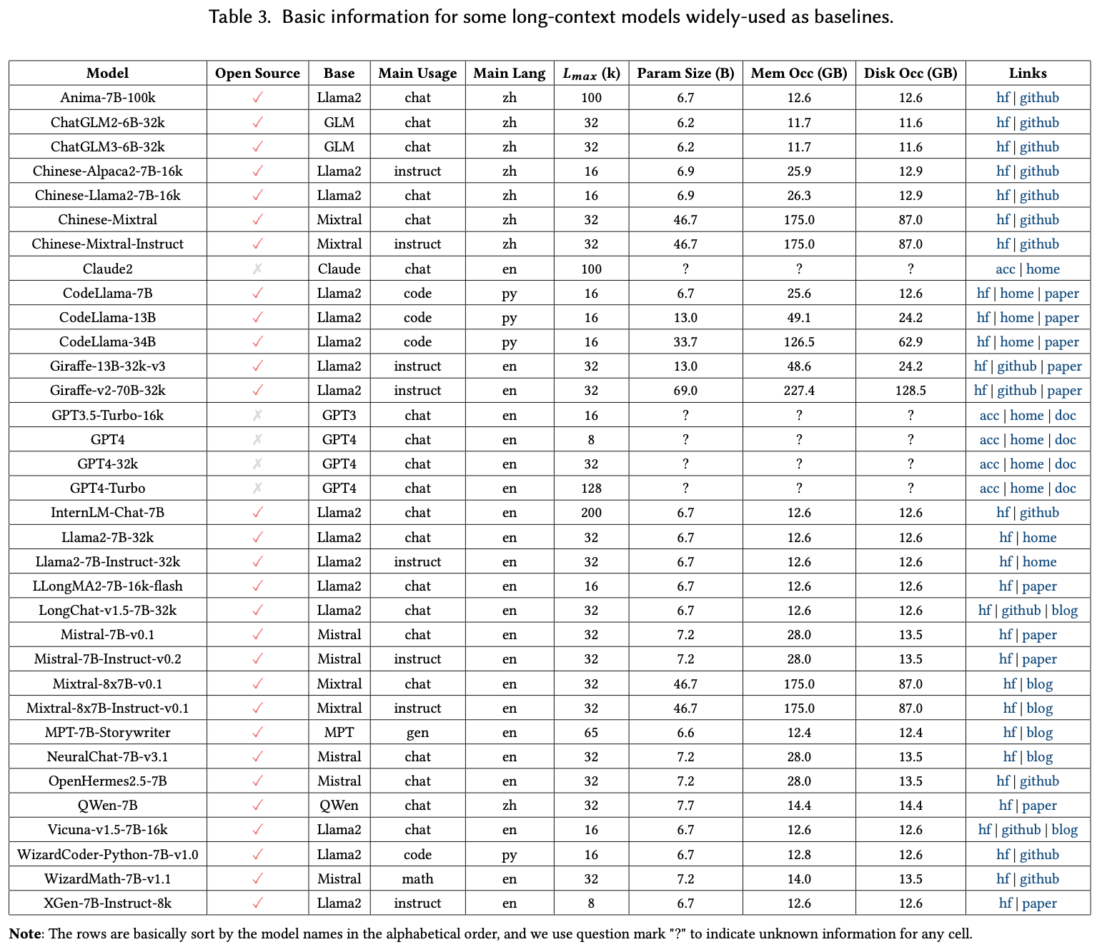
For Baselines, Table 3 gathers a list of pretrained/finetuned LLMs commonly, serving as baselines for evaluating long-context capabilities across various downstream tasks.

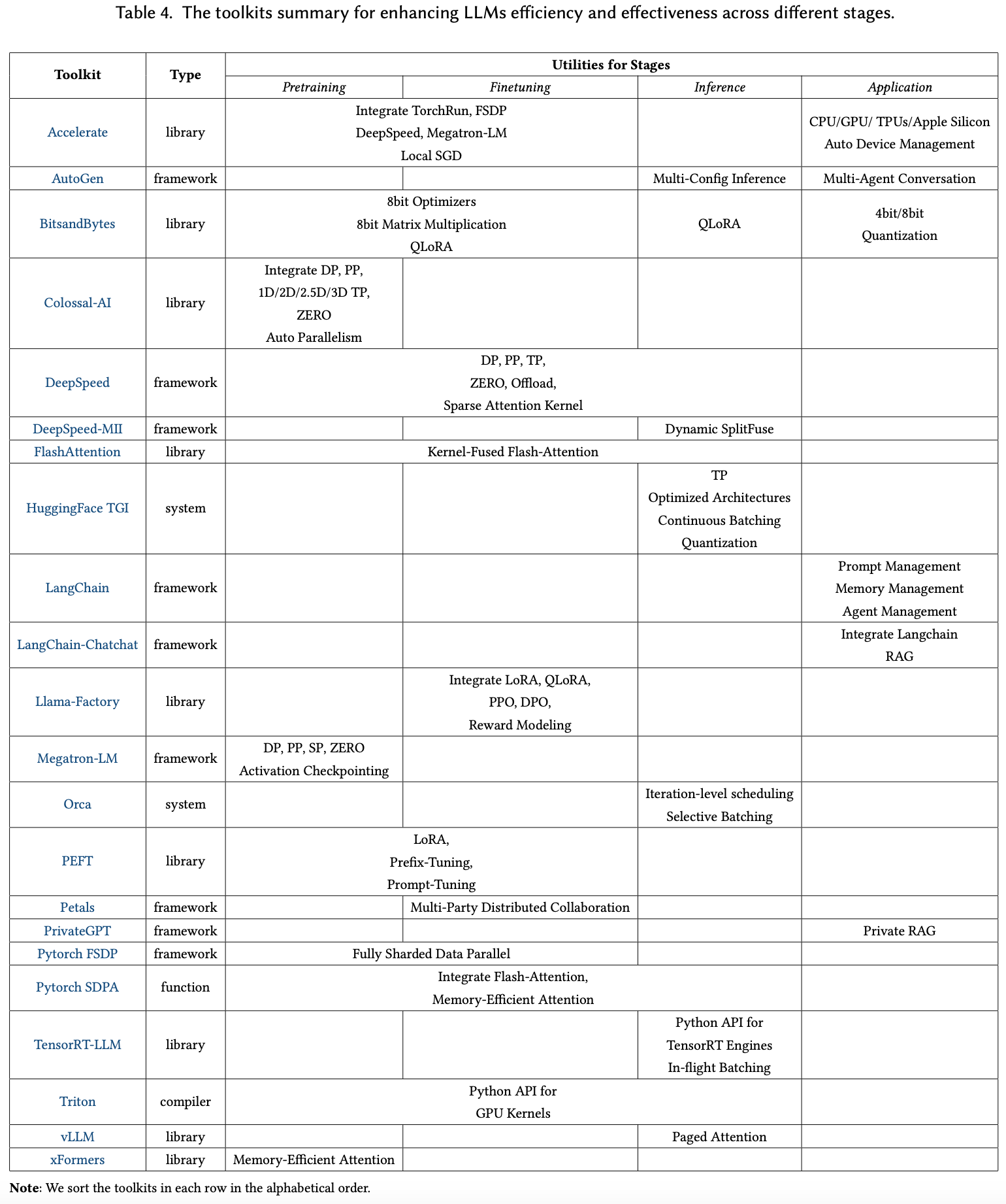
For Toolkit, Table 4 collects a diverse array of valuable toolkits to optimize the efficiency and effectiveness of LLMs across their development lifecycle.

FlashAttention: Fast and Memory-Efficient Exact Attention with IO-Awareness

Motivation

Transformers based on current attention architectures do not perform well when context length is beyond a threshold. The first motivation of this work is that designing a transformer architecture that can model longer sequence data has the following potential applications:

1. In NLP tasks, a large context allows the LLM to read books, plays and instruction manuals before generating a response.
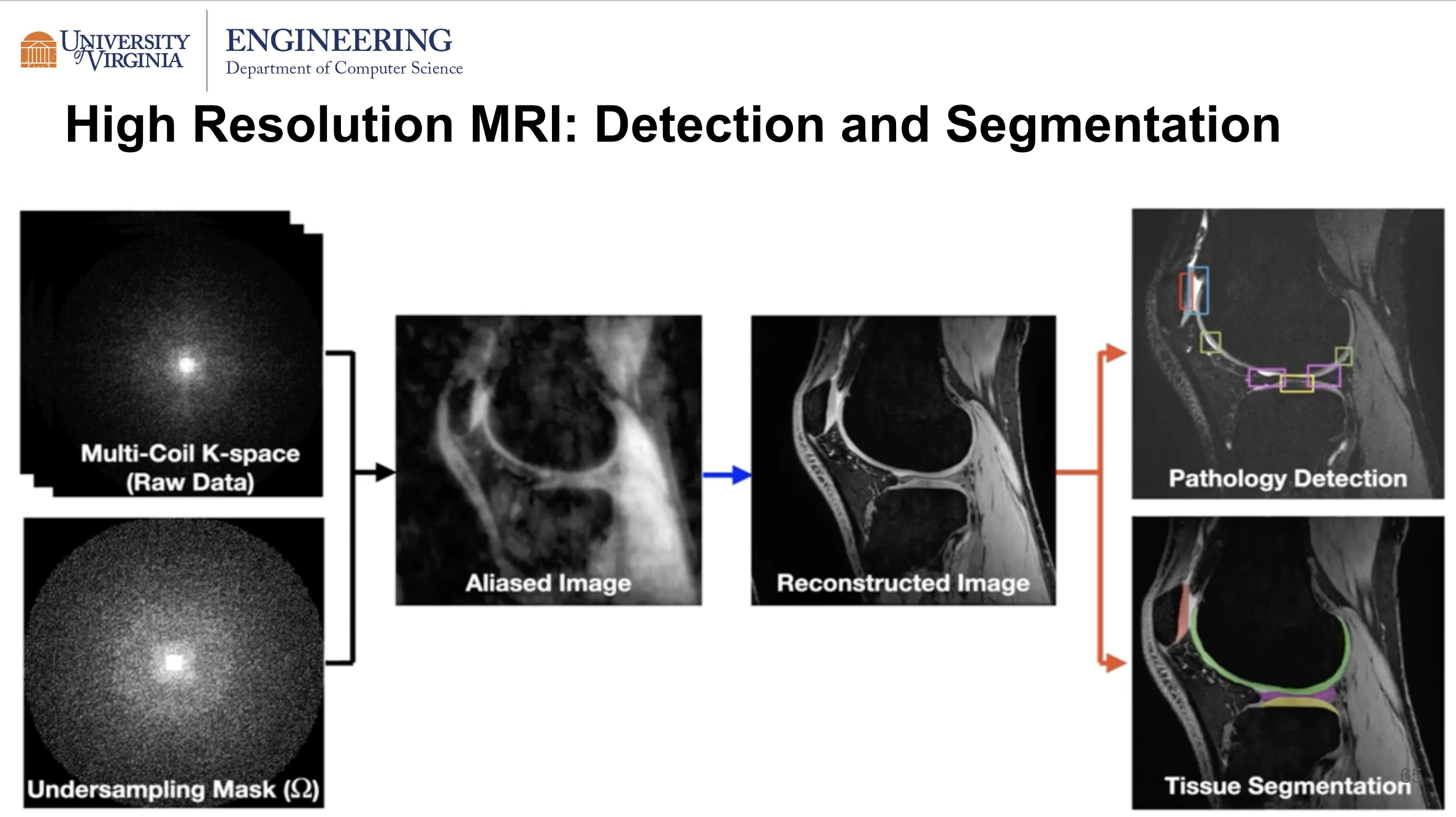
2. In computer vision, higher resolution images require the attention architecture to be capable of handling longer sequences. In the case of high resolution MRI as shown in the slide below, if the transformer is able to generate a high resolution image, it can improve the performance of downstream tasks such as pathology detection or tissue segmentation.
3. Other types of natural sequence data such as time-series data, audio data, video data and medical imaging also require the transformer to perform well on much longer sequences.

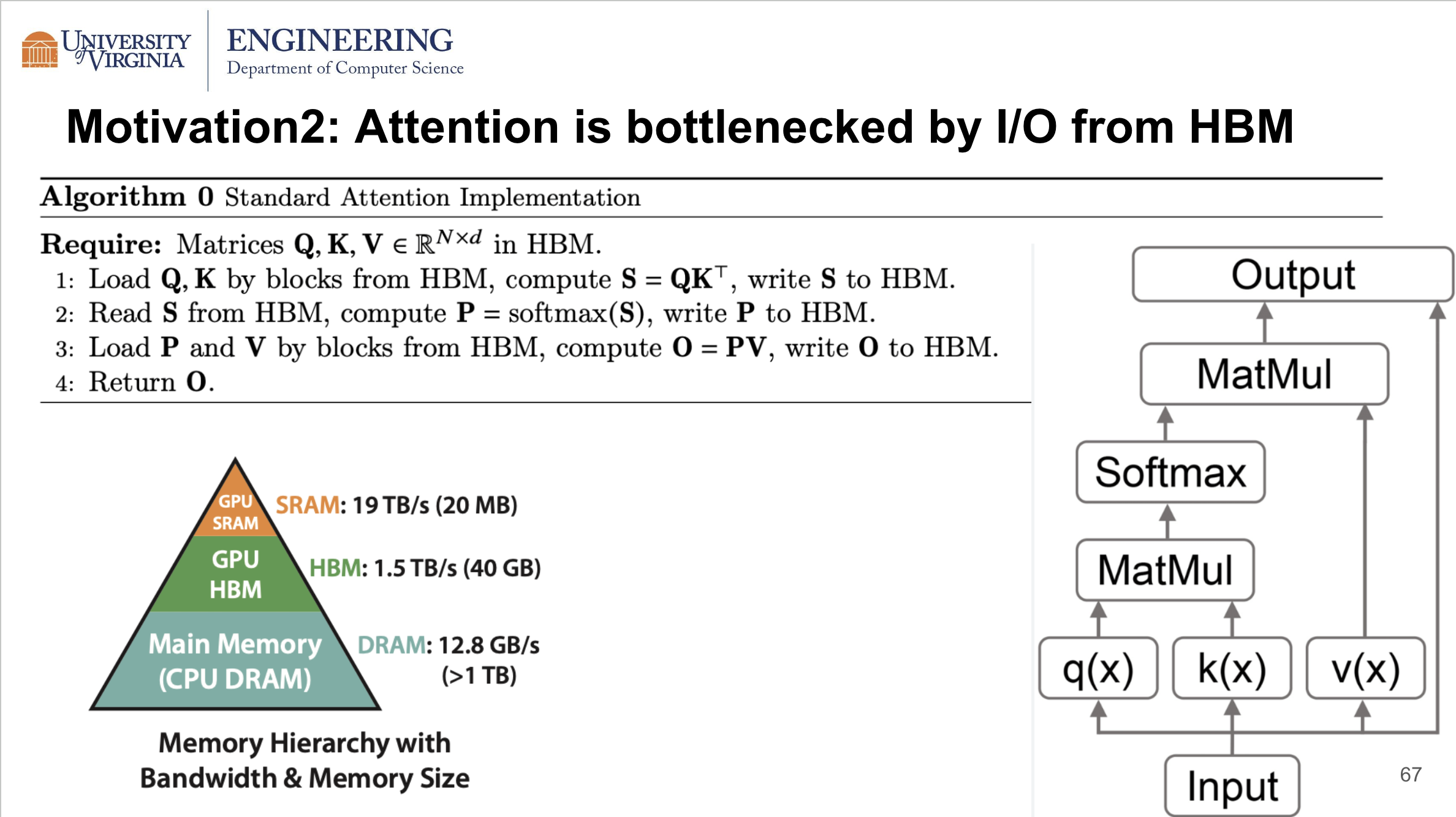
The second motivation of the work is that the attention computation is bottlenecked by the I/O from High Bandwidth Memory (HBM), which is large in size but relatively slow compared to SRAM. As an example, A100 offers 40GB HBM or 80GB HBM, but its bandwidth is only 1/10 of that of SRAM. The standard attention computation, as shown in the slide below, however, requires numerous writing to and reading from HBM for intermediate values such as the attention matrix throughout the computation, which makes I/O from HBM the bottleneck of the attention computation.

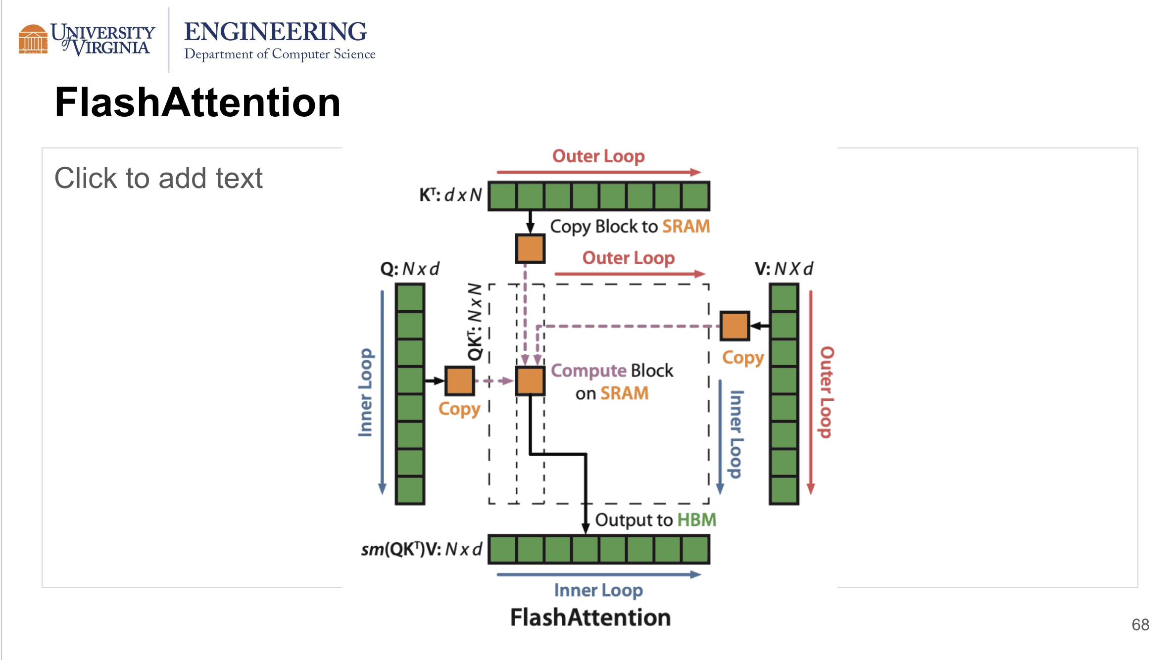
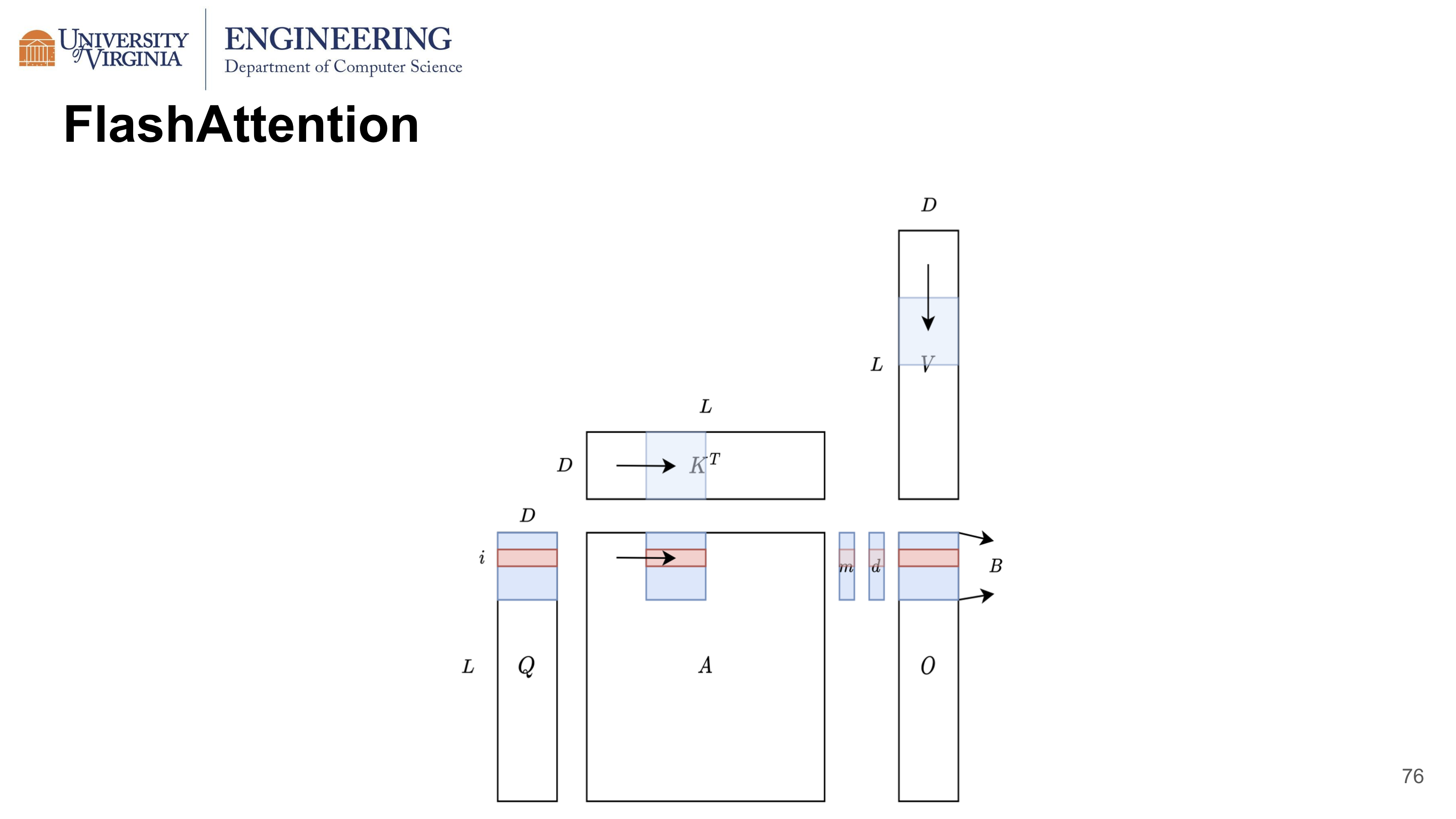
FlashAttention Algorithm

FlashAttention is fast, memory efficient and an exact computation of attention. FlashAttention is I/O aware and aims to reduce number of times needed to read and write to HBM. It computes the attention block by block. When computing each output block, all four blocks from Q, K, V and Output can be stored in SRAM. So we do not need to store the intermediate values to HBM. In addition, the overall SRAM memory footprint depends only on block size and head dimension and is not related to length. Instead of the entire attention matrix, since only a block is calculated each time, it can also handle longer sequences.

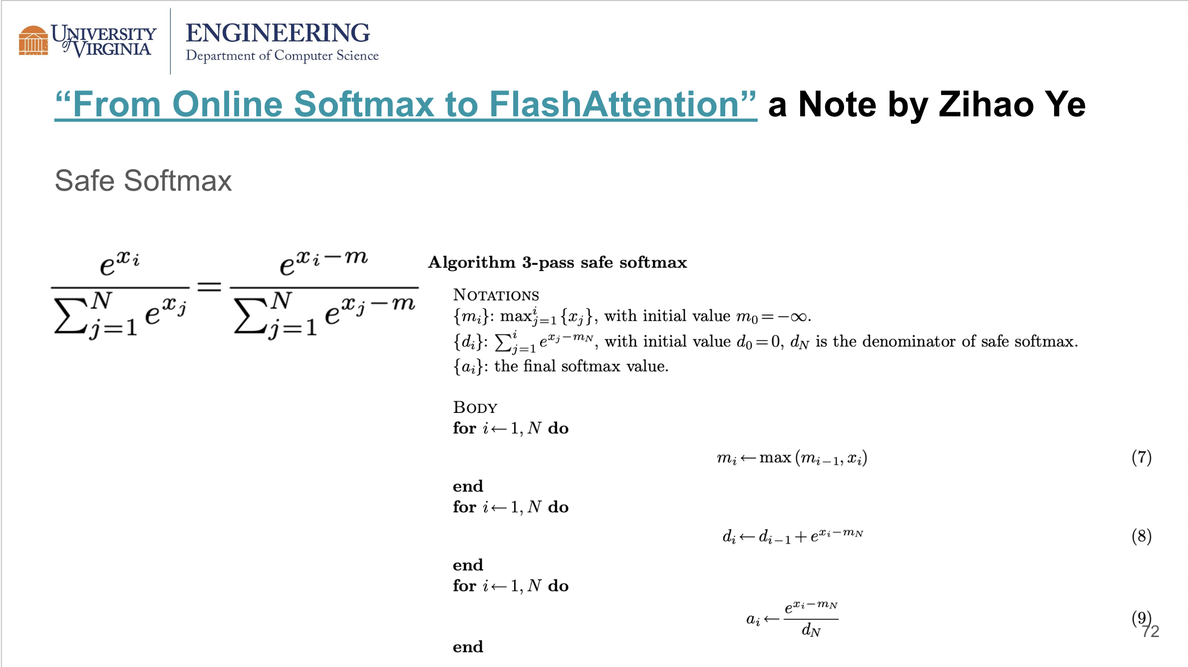
Flashattention is based on safe softmax and online softmax, which are simpler methods that may help us understand flashattention. To avoid numerical overflow, safe softmax subtracts m from the exponent which is the max over all input x, so that the exponential in softmax is less or equal to zero and safe to compute.

Safe Softmax requires a total of three passes. The first pass iteratively calculates a local maximum of the softmax imput, using the result from the previous iteration. When the for loop ends, the result will be the global maximum over all x. The second pass iteratively calculates the denominator using the global maximum from the previous pass. The final pass calculates the softmax using the denominator and the global max.

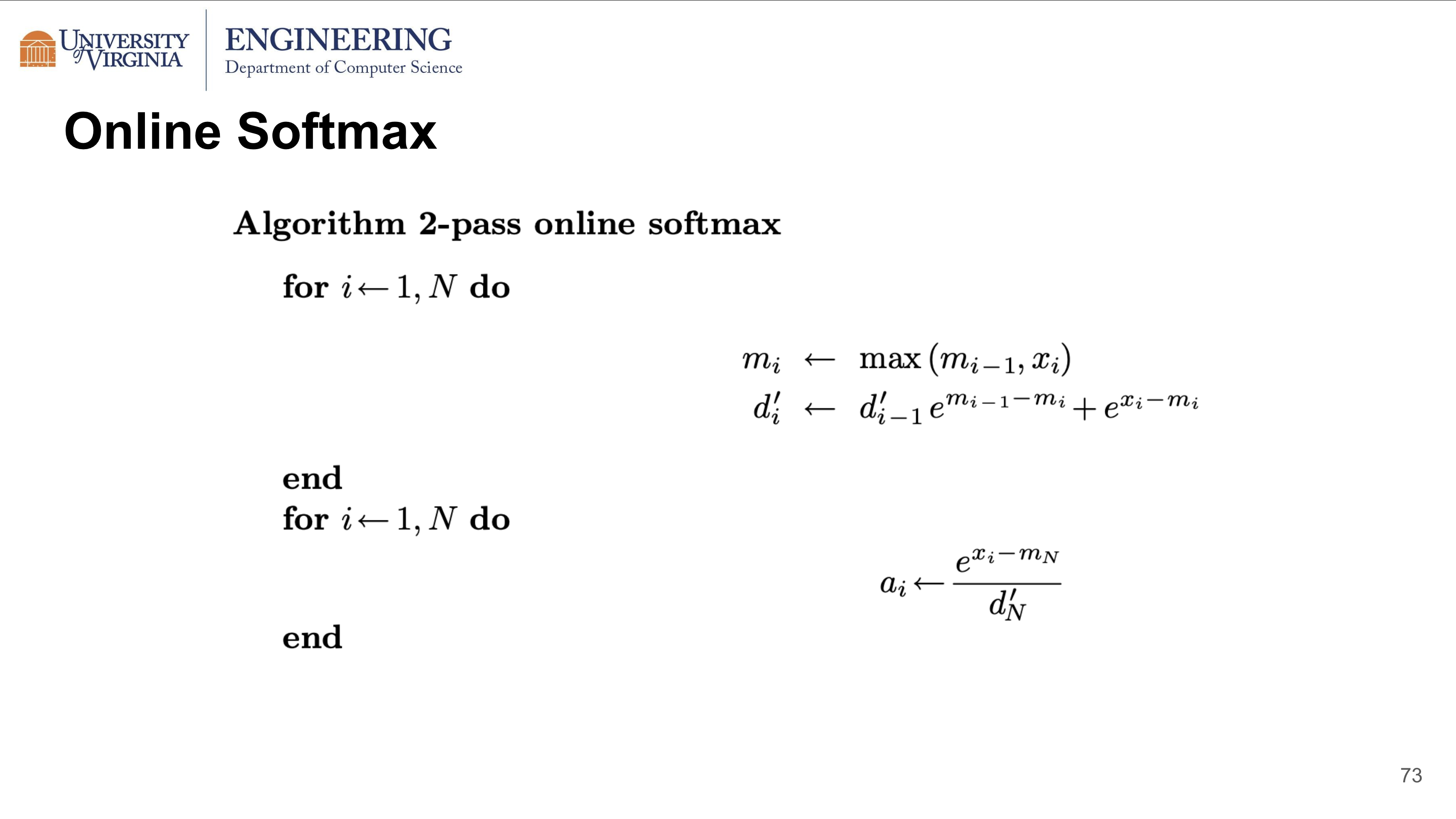
The online softmax reduces the computation from 3 passes to 2 passes. When updating the denominator of softmax, If we replace the global max and use the local max at iteration i with a scaling factor, we can calculate the max and the denominator together in 1 pass.

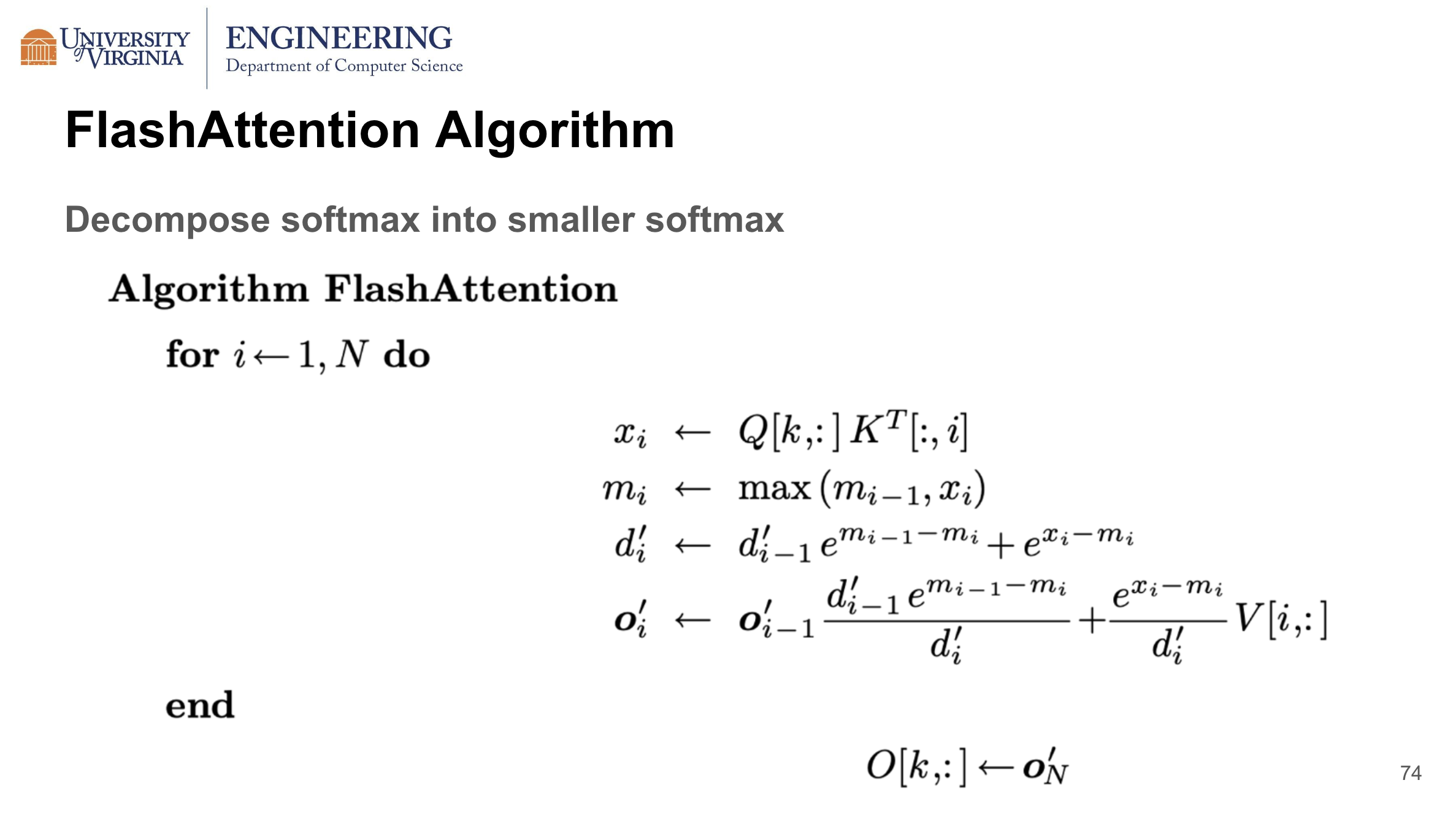
FlashAttention aims to reduce the calculation to 1 pass, and outputs attention instead of softmax in the previous two algorithms. Attention requires an additional calculation: a matrix multiplication of softmax and value V to obtain the output O. FlashAttention perform such calculation by breaking down softmax into smaller softmax. Here in the slide below, the output is updated in two terms. The first term is the output computed from the previous iteration times a scaling factor. The second term can be considered as a small softmax times a row of V. By updating the output in this iterative manner, FlashAttention can further reduce the computation to 1 pass.

This only calculating one row of Q, V and one column of K each time. To make full use of the SRAM fast cache memory, we can treat many rows together as blocks, and calculate the attention block by block. We are using a largest block size that can fit four blocks of Q, K, V, O onto the SRAM. For a particular block from Q, we iterate through all blocks from K transpose and V, while maintaining two columns of max and denominator. After the iterations, the result will obtain an exact block of output. In this procedure, FlashAttention calculates the attention in a block by block manner.

Evaluation

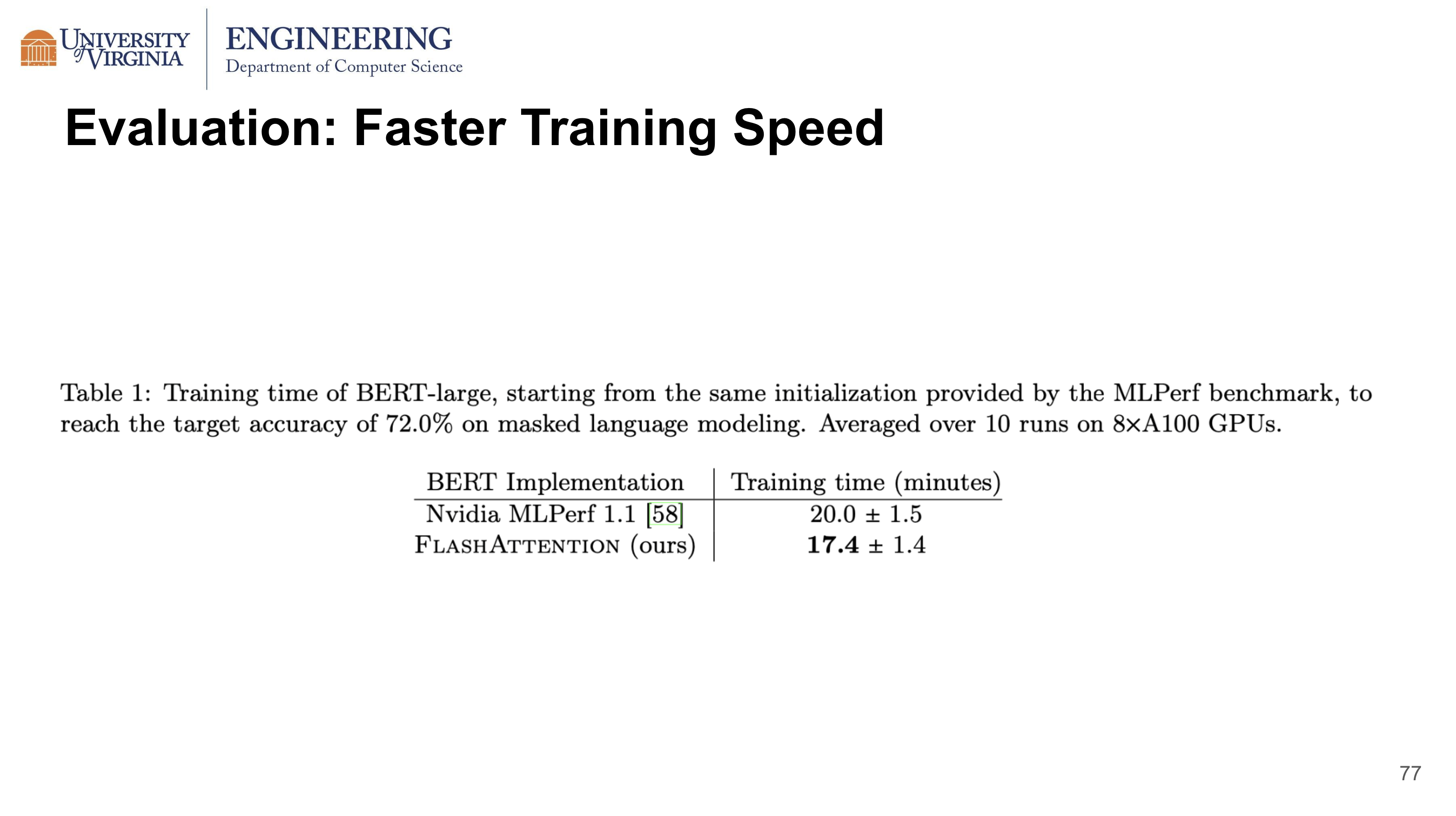
When both training a BERT-large model on a single node, FlashAttention is demonstrated to require 15% less training time than Nvidia’s attention implementation.

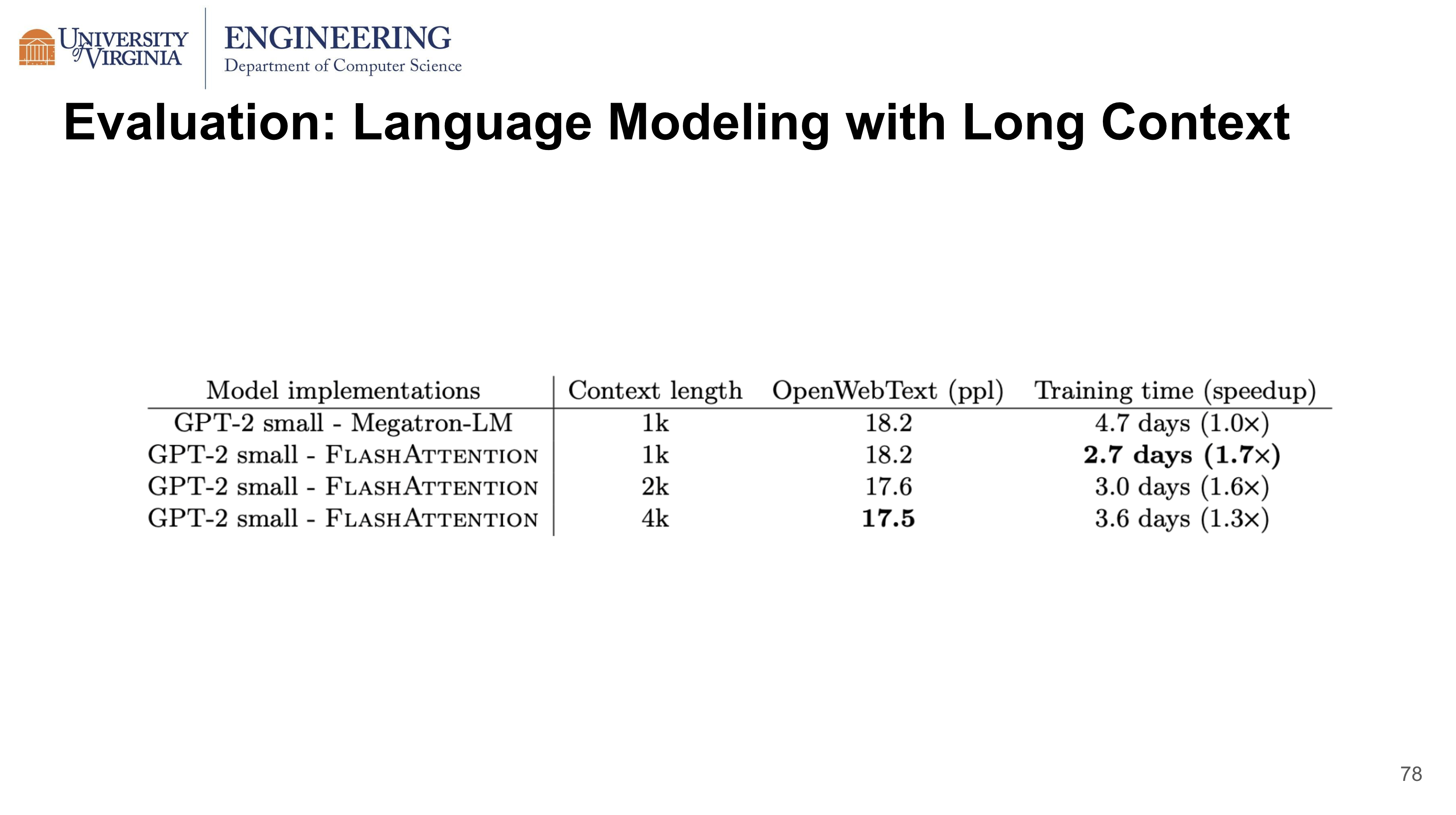
When training GPT-2 small, compared to Megatron-LM, FlashAttention supports 4 times longer the context length, is still being 30% faster while achieving 0.7 better perplexity.

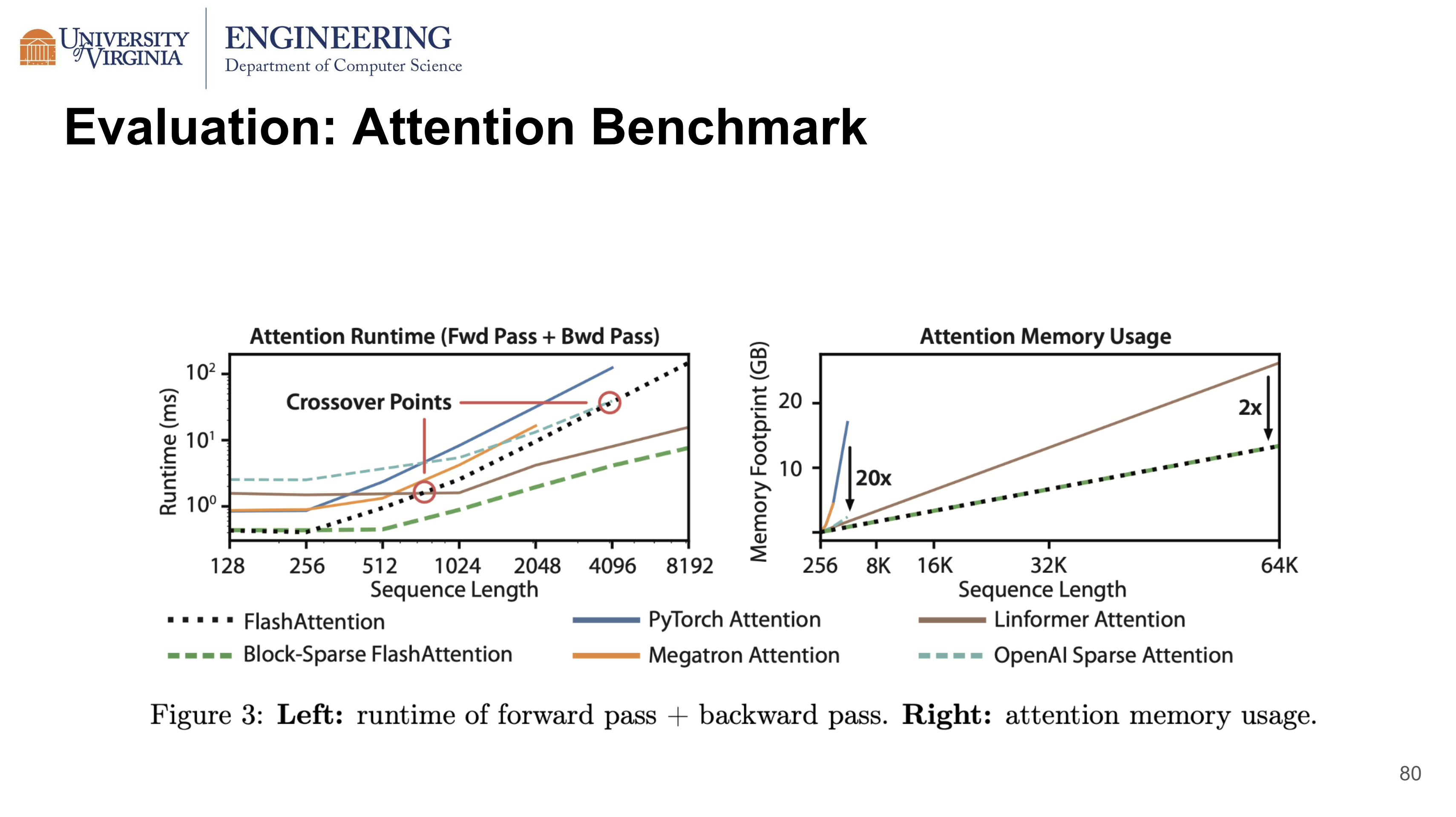
Being an exact attention implementation, FlashAttention is not only faster than PyTorch Attention, but also faster than OpenAI Sparse Attention, when the context length is less than 4096. It is slower than Linformer Attention, which is an approximation method using low-rank matrix. In terms of memory usage, it requires 2x less memory than Linformer Attention, and 20x less memory than Pytorch Attention.

Limitations and Future Directions

Compiling to CUDA. The current implementation requires writing a new CUDA kernel in low-level language use, and may not transfer to other GPU architectures. These limitations suggest a need to write attention algorithms in high-level language such as PyTorch.

IO-Aware Deep Learning. The IO-aware approach can be potentially extend to every layer in a deep network.

Multi-GPU IO-Aware Methods. The current algorithm is designed for a single GPU node and does not take data transfer across multiple GPU into consideration. The authors hope to inspire future work to design attention computation that is parallelizable across multiple GPUs.